Real-time object detection with YOLO

Object detection is one of the classical problems in computer vision:

Recognize what the objects are inside a given image and also where they are in the image.

Detection is a more complex problem than classification, which can also recognize objects but doesn’t tell you exactly where the object is located in the image — and it won’t work for images that contain more than one object.

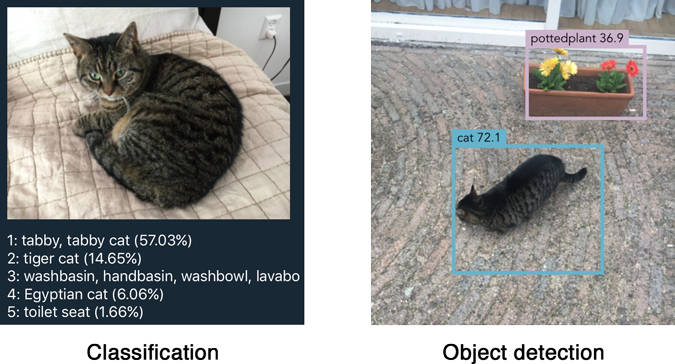
YOLO is a clever neural network for doing object detection in real-time.

In this blog post I’ll describe what it took to get the “tiny” version of YOLOv2 running on iOS using Metal Performance Shaders.

Before you continue, make sure to watch the awesome YOLOv2 trailer. 😎

How YOLO works

You can take a classifier like VGGNet or Inception and turn it into an object detector by sliding a small window across the image. At each step you run the classifier to get a prediction of what sort of object is inside the current window. Using a sliding window gives several hundred or thousand predictions for that image, but you only keep the ones the classifier is the most certain about.

This approach works but it’s obviously going to be very slow, since you need to run the classifier many times. A slightly more efficient approach is to first predict which parts of the image contain interesting information — so-called region proposals — and then run the classifier only on these regions. The classifier has to do less work than with the sliding windows but still gets run many times over.

YOLO takes a completely different approach. It’s not a traditional classifier that is repurposed to be an object detector. YOLO actually looks at the image just once (hence its name: You Only Look Once) but in a clever way.

YOLO divides up the image into a grid of 13 by 13 cells:

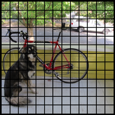
Each of these cells is responsible for predicting 5 bounding boxes. A bounding box describes the rectangle that encloses an object.

YOLO also outputs a confidence score that tells us how certain it is that the predicted bounding box actually encloses some object. This score doesn’t say anything about what kind of object is in the box, just if the shape of the box is any good.

The predicted bounding boxes may look something like the following (the higher the confidence score, the fatter the box is drawn):

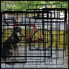
For each bounding box, the cell also predicts a class. This works just like a classifier: it gives a probability distribution over all the possible classes. The version of YOLO we’re using is trained on the PASCAL VOC dataset, which can detect 20 different classes such as:

• bicycle
• boat
• car
• cat
• dog
• person
• and so on…

The confidence score for the bounding box and the class prediction are combined into one final score that tells us the probability that this bounding box contains a specific type of object. For example, the big fat yellow box on the left is 85% sure it contains the object “dog”:

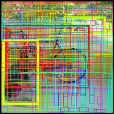
Since there are 13×13 = 169 grid cells and each cell predicts 5 bounding boxes, we end up with 845 bounding boxes in total. It turns out that most of these boxes will have very low confidence scores, so we only keep the boxes whose final score is 30% or more (you can change this threshold depending on how accurate you want the detector to be).

The final prediction is then:

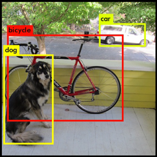
From the 845 total bounding boxes we only kept these three because they gave the best results. But note that even though there were 845 separate predictions, they were all made at the same time — the neural network just ran once. And that’s why YOLO is so powerful and fast.

(The above pictures are from pjreddie.com.)

The neural network

The architecture of YOLO is simple, it’s just a convolutional neural network:

Layer         kernel  stride  output shape
---------------------------------------------
Input                          (416, 416, 3)
Convolution    3×3      1      (416, 416, 16)
MaxPooling     2×2      2      (208, 208, 16)
Convolution    3×3      1      (208, 208, 32)
MaxPooling     2×2      2      (104, 104, 32)
Convolution    3×3      1      (104, 104, 64)
MaxPooling     2×2      2      (52, 52, 64)
Convolution    3×3      1      (52, 52, 128)
MaxPooling     2×2      2      (26, 26, 128)
Convolution    3×3      1      (26, 26, 256)
MaxPooling     2×2      2      (13, 13, 256)
Convolution    3×3      1      (13, 13, 512)
MaxPooling     2×2      1      (13, 13, 512)
Convolution    3×3      1      (13, 13, 1024)
Convolution    3×3      1      (13, 13, 1024)
Convolution    1×1      1      (13, 13, 125)
---------------------------------------------

This neural network only uses standard layer types: convolution with a 3×3 kernel and max-pooling with a 2×2 kernel. No fancy stuff. There is no fully-connected layer in YOLOv2.

The very last convolutional layer has a 1×1 kernel and exists to reduce the data to the shape 13×13×125. This 13×13 should look familiar: that is the size of the grid that the image gets divided into.

So we end up with 125 channels for every grid cell. These 125 numbers contain the data for the bounding boxes and the class predictions. Why 125? Well, each grid cell predicts 5 bounding boxes and a bounding box is described by 25 data elements:

• x, y, width, height for the bounding box’s rectangle
• the confidence score
• the probability distribution over the 20 classes

Using YOLO is simple: you give it an input image (resized to 416×416 pixels), it goes through the convolutional network in a single pass, and comes out the other end as a 13×13×125 tensor describing the bounding boxes for the grid cells. All you need to do then is compute the final scores for the bounding boxes and throw away the ones scoring lower than 30%.

Converting to Metal

The architecture I just described is for Tiny YOLO, which is the version we’ll be using in the iOS app. The full YOLOv2 network has three times as many layers and is a bit too big to run fast enough on current iPhones. Since Tiny YOLO uses fewer layers, it is faster than its big brother… but also a little less accurate.

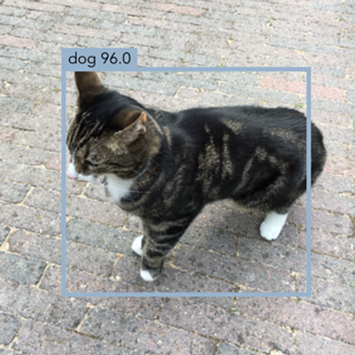
YOLO is written in Darknet, a custom deep learning framework from YOLO’s author. The downloadable weights are available only in Darknet format. Even though the source code for Darknet is available, I wasn’t really looking forward to spending a lot of time figuring out how it works.

Luckily for me, someone else already put in that effort and converted the Darknet models to Keras, my deep learning tool of choice. So all I had to do was run this “YAD2K” script to convert the Darknet weights to Keras format, and then write my own script to convert the Keras weights to Metal.

However, there was a small wrinkle… YOLO uses a regularization technique called batch normalization after its convolutional layers.

The idea behind “batch norm” is that neural network layers work best when the data is clean. Ideally, the input to a layer has an average value of 0 and not too much variance. This should sound familiar to anyone who’s done any machine learning because we often use a technique called “feature scaling” or “whitening” on our input data to achieve this.

Batch normalization does a similar kind of feature scaling for the data in between layers. This technique really helps neural networks perform better because it stops the data from deteriorating as it flows through the network.

To give you some idea of the effect of batch norm, here is a histogram of the output of the first convolution layer without and with batch normalization:

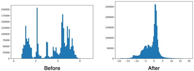
Batch normalization is important when training a deep network, but it turns out we can get rid of it at inference time. Which is a good thing because not having to do the batch norm calculations will make our app faster. And in any case, Metal does not have an MPSCNNBatchNormalization layer.

Batch normalization usually happens after the convolutional layer but before the activation function gets applied (a so-called “leaky” ReLU in the case of YOLO). Since both convolution and batch norm perform a linear transformation of the data, we can combine the batch normalization layer’s parameters with the weights for the convolution. This is called “folding” the batch norm layer into the convolution layer.

Long story short, with a bit of math we can get rid of the batch normalization layers but it does mean we have to change the weights of the preceding convolution layer.

A quick recap of what a convolution layer calculates: if x is the pixels in the input image and w is the weights for the layer, then the convolution basically computes the following for each output pixel:

out[j] = x[i]*w[0] + x[i+1]*w[1] + x[i+2]*w[2] + ... + x[i+k]*w[k] + b

This is a dot product of the input pixels with the weights of the convolution kernel, plus a bias value b.

And here’s the calculation performed by the batch normalization to the output of that convolution:

        gamma * (out[j] - mean)
bn[j] = ---------------------- + beta
            sqrt(variance)

It subtracts the mean from the output pixel, divides by the variance, multiplies by a scaling factor gamma, and adds the offset beta. These four parameters — mean, variance, gamma, and beta — are what the batch normalization layer learns as the network is trained.

To get rid of the batch normalization, we can shuffle these two equations around a bit to compute new weights and bias terms for the convolution layer:

           gamma * w
w_new = --------------
        sqrt(variance)

        gamma*(b - mean)
b_new = ---------------- + beta
         sqrt(variance)

Performing a convolution with these new weights and bias terms on input x will give the same result as the original convolution plus batch normalization.

Now we can remove this batch normalization layer and just use the convolutional layer, but with these adjusted weights and bias terms w_new and b_new. We repeat this procedure for all the convolutional layers in the network.

Once we’ve folded all the batch norm layers into their preceding convolution layers, we can convert the weights to Metal. This is a simple matter of transposing the arrays (Keras stores them in a different order than Metal) and writing them out to binary files of 32-bit floating point numbers.

If you’re curious, check out the conversion script yolo2metal.py for more details. To test that the folding works the script creates a new model without batch norm but with the adjusted weights, and compares it to the predictions of the original model.

The iOS app

Of course I used Forge to build the iOS app. 😂 You can find the code in the YOLO folder. To try it out: download or clone Forge, open Forge.xcworkspace in Xcode 8.3 or later, and run the YOLO target on an iPhone 6 or up.

The easiest way to test the app is to point your iPhone at some YouTube videos:

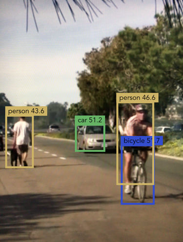
The interesting code is in YOLO.swift. First this sets up the convolutional network:

let leaky = MPSCNNNeuronReLU(device: device, a: 0.1)

let input = Input()

let output = input
         --> Resize(width: 416, height: 416)
         --> Convolution(kernel: (3, 3), channels: 16, padding: true, activation: leaky, name: "conv1")
         --> MaxPooling(kernel: (2, 2), stride: (2, 2))
         --> Convolution(kernel: (3, 3), channels: 32, padding: true, activation: leaky, name: "conv2")
         --> MaxPooling(kernel: (2, 2), stride: (2, 2))
         --> ...and so on...

The input from the camera gets rescaled to 416×416 pixels and then goes into the convolutional and max-pooling layers. This is very similar to how any other convnet operates.

The interesting thing is what happens with the output. Recall that the output of the convnet is a 13×13×125 tensor: there are 125 channels of data for each of the cells in the grid that is overlaid on the image. These 125 numbers contain the bounding boxes and class predictions, and we need to sort these out somehow. This happens in the function fetchResult().

Here is how fetchResult() works:

public func fetchResult(inflightIndex: Int) -> NeuralNetworkResult<Prediction> {
  let featuresImage = model.outputImage(inflightIndex: inflightIndex)
  let features = featuresImage.toFloatArray()

The output from the convolutional network is in the form of an MPSImage. We first convert this to an array of Float values called features, to make it a little easier to work with.

The main body of fetchResult() is a huge nested loop. It looks at all of the grid cells and the five predictions for each cell:

  for cy in 0..<13 {
    for cx in 0..<13 {
      for b in 0..<5 {
         . . .
      }
    }
  }

Inside this loop we compute the bounding box b for grid cell (cy, cx).

First we read the x, y, width, and height for the bounding box from the features array, as well as the confidence score:

let channel = b*(numClasses + 5)
let tx = features[offset(channel, cx, cy)]
let ty = features[offset(channel + 1, cx, cy)]
let tw = features[offset(channel + 2, cx, cy)]
let th = features[offset(channel + 3, cx, cy)]
let tc = features[offset(channel + 4, cx, cy)]

The offset() helper function is used to find the proper place in the array to read from. Metal stores its data in texture slices in groups of 4 channels at a time, which means the 125 channels are not stored consecutively but are scattered all over the place. (See the code for an in-depth explanation.)

We still need to do some processing on these five numbers tx, ty, tw, th, tc as they are in a bit of a weird format. If you’re wondering where these formulas come from, they’re given in the paper (it’s a side effect of how the network was trained).

let x = (Float(cx) + Math.sigmoid(tx)) * 32
let y = (Float(cy) + Math.sigmoid(ty)) * 32

let w = exp(tw) * anchors[2*b    ] * 32
let h = exp(th) * anchors[2*b + 1] * 32

let confidence = Math.sigmoid(tc)

Now x and y represent the center of the bounding box in the 416×416 image that we used as input to the neural network; w and h are the width and height of the box in that same image space. The confidence value for the bounding box is given by tc and we used the logistic sigmoid to turn this into a percentage.

We now have our bounding box and we know how confident YOLO is that this box actually contains an object. Next, let’s look at the class predictions to see what kind of object YOLO thinks is inside the box:

var classes = [Float](repeating: 0, count: numClasses)
for c in 0..<numClasses {
  classes[c] = features[offset(channel + 5 + c, cx, cy)]
}
classes = Math.softmax(classes)

let (detectedClass, bestClassScore) = classes.argmax()

Recall that 20 of the channels in the features array contain the class predictions for this bounding box. We read those into a new array, classes. As is usual for classifiers, we take the softmax to turn the array into a probability distribution. And then we pick the class with the largest score as the winner.

Now we can compute the final score for this bounding box — for example, “I’m 85% sure this bounding box contains a dog”. As there are 845 bounding boxes in total, we only want to keep the ones whose combined score is over a certain threshold.

let confidenceInClass = bestClassScore * confidence
if confidenceInClass > 0.3 {
  let rect = CGRect(x: CGFloat(x - w/2), y: CGFloat(y - h/2),
                    width: CGFloat(w), height: CGFloat(h))

  let prediction = Prediction(classIndex: detectedClass,
                              score: confidenceInClass,
                              rect: rect)
  predictions.append(prediction)
}

The above code is repeated for all the cells in the grid. When the loop is over, we have a predictions array with typically 10 to 20 predictions in it.

We already filtered out any bounding boxes that have very low scores, but there still may be boxes that overlap too much with others. Therefore, the last thing we do in fetchResult() is a technique called non-maximum suppression to prune those duplicate bounding boxes.

  var result = NeuralNetworkResult<Prediction>()
  result.predictions = nonMaxSuppression(boxes: predictions,
                                         limit: 10, threshold: 0.5)
  return result
}

The algorithm used by the nonMaxSuppression() function is quite simple:

1. Start with the bounding box that has the highest score.
2. Remove any remaining bounding boxes that overlap it more than the given threshold amount (i.e. more than 50%).
3. Go to step 1 until there are no more bounding boxes left.

This removes any bounding boxes that overlap too much with other boxes that have a higher score. It only keeps the best ones.

And that’s pretty much all there is to it: a regular convolutional network and a bit of postprocessing of the results afterwards.

How well does it work?

The YOLO website claims that Tiny YOLO can do up to 200 frames per second. But of course that is on a fat desktop GPU, not on a mobile device. So how fast does it run on an iPhone?

On my iPhone 6s it takes about 0.15 seconds to process a single image. That is only 6 FPS, barely fast enough to call it realtime. If you point the phone at a car driving by, you can see the bounding box trailing a little behind the car. Still, I’m impressed this technique works at all. 😁

I think a major slowdown is caused by the convolutional layers that have 512 and 1024 output channels. From my experiments it seems that MPSCNNConvolution has more trouble with small images that have many channels than with large images that have fewer channels.

One thing I’m interested in trying is to take a different network architecture, such as SqueezeNet, and retrain this network to predict the bounding boxes in its last layer. In other words, to take the YOLO ideas and put them on top of a smaller and faster convnet. Will the increase in speed be worth the loss in accuracy?

Credits

To learn more about YOLO, check out these papers by its inventors:

• You Only Look Once: Unified, Real-Time Object Detection by Joseph Redmon, Santosh Divvala, Ross Girshick, Ali Farhadi (2015)
• YOLO9000: Better, Faster, Stronger by Joseph Redmon and Ali Farhadi (2016)

My implementation was based in part on the TensorFlow Android demo TF Detect, Allan Zelener’s YAD2K, and the original Darknet code.