
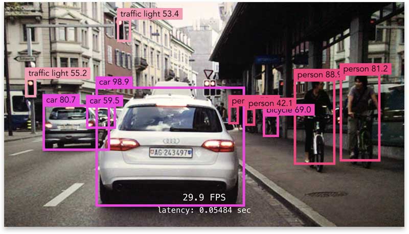
Object detection is the computer vision technique for finding objects of interest in an image:
This is more advanced than classification, which only tells you what the “main subject” of the image is — whereas object detection can find multiple objects, classify them, and locate where they are in the image.
An object detection model predicts bounding boxes, one for each object it finds, as well as classification probabilities for each object.
It’s common for object detection to predict too many bounding boxes. Each box also has a confidence score that says how likely the model thinks this box really contains an object. As a post-processing step we filter out the boxes whose score falls below a certain threshold (also called non-maximum suppression).
Object detection is more tricky than classification. One of the problems you’ll encounter is that a training image can have anywhere from zero to dozens of objects in them, and the model may output more than one prediction, so how do you figure out which prediction should be compared to which ground-truth bounding box in the loss function?
Since I work with mobile, I’m mostly interested in one-stage object detectors.
A high-end model like Faster R-CNN first generates so-called region proposals — areas of the image that potentially contain an object — and then it makes a separate prediction for each of these regions. That works well but it’s also quite slow as it requires running the detection and classification portion of the model multiple times.
A one-stage detector, on the other hand, requires only a single pass through the neural network and predicts all the bounding boxes in one go. That is much faster and much more suitable for mobile devices. The most common examples of one-stage object detectors are YOLO, SSD, SqueezeDet, and DetectNet.
Unfortunately, the research papers for these models leave out a lot of important technical details, and there aren’t many in-depth blog posts about training such models either. So to figure out these details, I spent a lot of time trying to make sense out of the papers, digging through other people’s source code, and training my own object detectors from scratch.
In this (long!) blog post I’ll try to explain how these one-stage detectors work and how they are trained and evaluated.
Note: You may also be interested in my other posts about object detection with YOLO on iOS.
By the way, YOLO stands for You Only Look Once, while SSD stands for Single-Shot MultiBox Detector (I guess SSMBD wasn’t a great acronym).
Why object detection is tricky
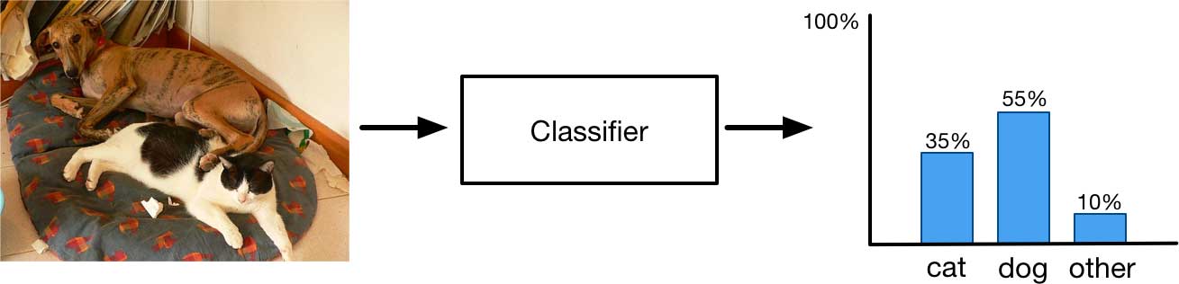
A classifier takes an image as input and produces a single output, the probability distribution over the classes. But this only gives you a summary of what is in the image as a whole, it doesn’t work so well when the image has multiple objects of interest.
On the following image, a classifier might recognize that the image contains a certain amount of “cat-ness” and certain amount of “dog-ness” but that’s the best it can do.
An object detection model, on the other hand, will tell you where the individual objects are by predicting a bounding box for each object:
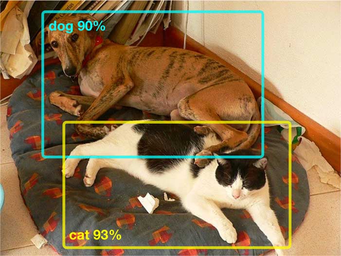
Since it can now focus on classifying the thing inside the bounding box and ignore everything outside, the model is able to give much more confident predictions for the individual objects.
If your dataset comes with bounding box annotations (the so-called ground-truth boxes), it’s pretty easy to add a localization output to your model. Simply predict an additional 4 numbers, one for each corner of the bounding box.

Now the model has two outputs:
- the usual probability distribution for the classification result, and
- a bounding box regression.
The loss function for the model simply adds the regression loss for the bounding box to the cross-entropy loss for the classification, usually with the mean squared error (MSE):
outputs = model.forward_pass(image)
class_pred = outputs[0]
bbox_pred = outputs[1]
class_loss = cross_entropy_loss(class_pred, class_true)
bbox_loss = mse_loss(bbox_pred, bbox_true)
loss = class_loss + bbox_loss
optimize(loss)
Now you use SGD to optimize the model as usual, with this combined loss, and it actually works pretty well. Here is an example prediction:

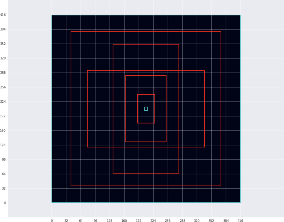
The model has correctly found the class for this object (dog) and also its location in the image. The red box is the ground-truth while the cyan box is the prediction. It’s not a perfect match, but pretty close.
Note: The score of 52.14% given here is a combination of the class score, which was 82.16% dog, and a confidence score of how likely it is that the bounding box really contains an object, which was 63.47%.
To score how well the predicted box matches the ground-truth we can compute the IOU (or intersection-over-union, also known as the Jaccard index) between the two bounding boxes.
The IOU is a number between 0 and 1, with larger being better. Ideally, the predicted box and the ground-truth have an IOU of 100% but in practice anything over 50% is usually considered to be a correct prediction. For the above example the IOU is 74.9% and you can see the boxes are a good match.
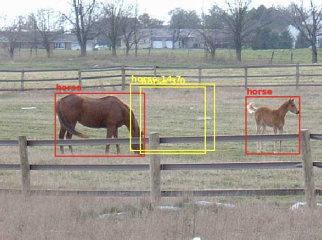
Using a regression output to predict a single bounding box gives good results. However, just like classification doesn’t work so well when there’s more than one object of interest in the image, so fails this simple localization scheme:
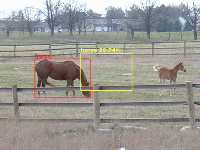
The model can predict only one bounding box and so it has to choose one of the objects, but instead the box ends up somewhere in the middle. Actually what happens here makes perfect sense: the model knows there are two objects but it has only one bounding box to give away, so it compromises and puts the predicted box in between the two horses. The size of the box is also halfway between the sizes of the two horses.
Note: You might perhaps expect that the model would now draw the box around both objects, but that doesn’t happen because it has not been trained to do so. The ground-truth annotations in the dataset are always drawn around individual objects, not around groups of objects.
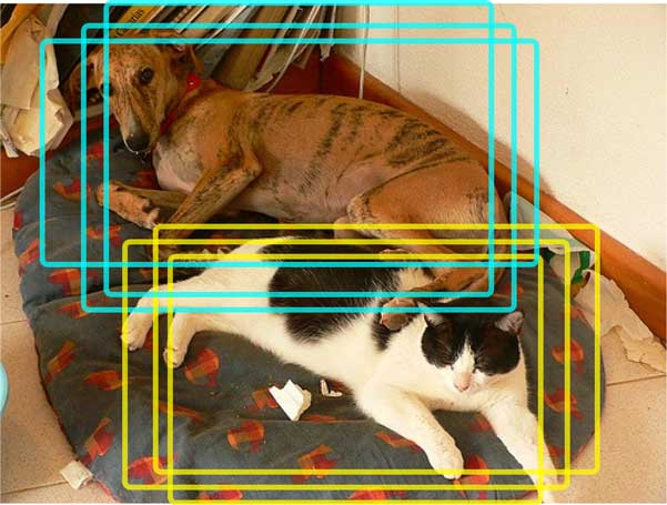
You may think, “This sounds easy enough to solve, let’s just add more bounding box detectors by giving the model additional regression outputs.” After all, if the model can predict N bounding boxes then it should be able find up to N objects, right? Sounds like a plan… but it doesn’t work. 🤕
Even with a model that has multiple of these detectors, we still get bounding boxes that all end up in the middle of the image:
Why does this happen? The problem is that the model doesn’t know which bounding box it should assign to which object, and to be safe it puts them both somewhere in the middle.
The model has no way to decide, “I can put bounding box 1 around the horse on the left, and bounding box 2 around the horse on the right.” Instead, each detector still tries to predict all of the objects rather than just one of them. Even though the model has N detectors, they don’t work together as a team. A model with multiple bounding box detectors still behaves exactly like the model that predicted only one bounding box.
What we need is some way to make the bounding box detectors specialize, so that each detector will try to predict only a single object, and different detectors will find different objects.
In a model that doesn’t specialize, each detector is supposed to be able to handle every possible kind of object at any possible location in the image. This is simply too much to ask… The model is now tempted to learn to predict boxes that are always in the center of the image because over the entire training set that actually minimizes the amount of mistakes it makes.
From the point of view of SGD, doing so gives a pretty good result on average, but it’s also not really a useful result in practice… and so we need to be smarter about how we train the model.
One-stage detectors such as YOLO, SSD, and DetectNet all solve this problem by assigning each bounding box detector to a specific position in the image. That way the detectors learn to specialize on objects in certain locations. For even better results, we can also let detectors specialize on the shapes and sizes of objects.
Enter the grid
Using a fixed grid of detectors is the main idea that powers one-stage detectors, and what sets them apart from region proposal-based detectors such as R-CNN.
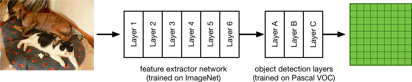
Let’s consider the simplest possible architecture for this kind of model. It exists of a base network that acts as a feature extractor. Like most feature extractors, it’s typically trained on ImageNet.
In the case of YOLO, the feature extractor takes in a 416×416 pixel image as input. SSD typically uses 300×300 images. These are larger than images for classification (typically something like 224×224) because we don’t want small details to get lost.
The base network can be anything, such as Inception or ResNet or YOLO’s DarkNet, but on mobile it makes sense to use a small, fast architecture such as SqueezeNet or MobileNet.
(In my own experiments, I took a MobileNet V1 feature extractor that was trained on 224×224 images. I scaled this up to 448×448 and then fine-tuned this network for 7 epochs on the ILSVRC 2012 dataset of 1.3 million images, using basic data augmentation such as random crops and color jittering. Re-training the feature extractor on these larger images makes the model work better on the 416×416 inputs used for object detection.)
On top of the feature extractor are several additional convolutional layers. These are fine-tuned to learn how to predict bounding boxes and class probabilities for the objects inside these bounding boxes. This is the object detection part of the model.
There are a number of common datasets for training object detectors. For the sake of this blog post we’ll be using the Pascal VOC dataset, which has 20 classes. So the first part of the neural network was trained on ImageNet, the second part on VOC.
When you look at the actual architectures of YOLO or SSD, they’re a little more complicated than this simple example network, with skip connections and so on, but we’ll get into that later. For now the above model will suffice, and can actually be used to build a fast and fairly accurate object detector. (It is very similar to the “Tiny YOLO” architecture that I’ve written about before.)
The output of the final layer is a feature map (the green thing in the illustration above). For our example model this is a 13×13 feature map with 125 channels.
Note: The number 13 here comes from the input size of 416 pixels and the fact that the particular base network used here has five pooling layers (or convolution layers with stride 2), which together scale down the input by a factor of 32, and 416 / 32 = 13. If you want a finer grid, for example 19×19, then the input image should be 19 × 32 = 608 pixels wide and tall (or you can use a network with a smaller stride).
We interpret this feature map as being a grid of 13 by 13 cells. The number is odd so that there is a single cell in the center. Each cell in the grid has 5 independent object detectors, and each of these detectors predicts a single bounding box.
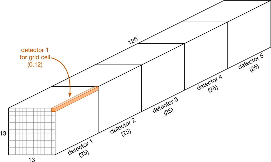
The key thing here is that the position of a detector is fixed: it can only detect objects located near that cell (in fact, the object’s center must be inside the grid cell). This is what lets us avoid the problem from the previous section, where detectors had too much freedom. With this grid, a detector on the left-hand side of the image will never predict an object that is located on the right-hand side.
Each object detector produces 25 numbers:
- 20 numbers containing the class probabilities
- 4 bounding box coordinates (center x, center y, width, height)
- 1 confidence score
Since there a 5 detectors per cell, and 5 × 25 = 125, that’s why we have 125 output channels.
Like with a regular classifier, the 20 numbers for the class probabilities have had a softmax applied to them. We can find the winning class by looking at the highest number. (Although it’s also common to treat this as multi-label classification, in which case the 20 classes are independent and we use sigmoid instead of softmax.)
The confidence score is a number between 0 and 1 (or 100%) and describes how likely the model thinks this predicted bounding box contains a real object. It’s also known as the “object-ness” score. Note that this score only says something about whether or not this is an object, but says nothing about what kind of object this is — that’s what the class probabilities are for.
This model always predicts the same number of bounding boxes: 13×13 cells times 5 detectors gives 845 predictions. Obviously, the vast majority of these predictions will be no good — after all, most images only contain a handful of objects at most, not over 800. The confidence score tells us which predicted boxes we can ignore.
Typically we’ll end up with a dozen or so predictions that the model thinks are good. Some of these will overlap — this happens because nearby cells may all make a prediction for the same object, and sometimes a single cell will make multiple predictions (although this is discouraged in training).
Having multiple, largely overlapping predictions is common with object detection. The standard postprocessing technique is to apply non-maximum suppression (NMS) to remove such duplicates. In short, NMS keeps the predictions with the highest confidence scores and removes any other boxes that overlap these by more than a certain threshold (say 60%).
Often we’ll only keep the 10 or so best predictions and discard the others. Ideally, we want to have only a single bounding box for each object in the image.
All right, that describes the basic pipeline for making object detection predictions using a grid. But why does it work?
Constraints are good
I’ve already mentioned that assigning each bounding box detector to a fixed position in the image is the trick that makes one-stage object detectors work. We use the 13×13 grid as a spatial constraint, to make it easier for the model to learn how to predict objects.
Using such (architectural) constraints is a useful technique for machine learning. In fact, convolutions are themselves a constraint too: a convolutional layer is really just a more restricted version of a fully-connected (FC) layer. (This is why you can implement convolutions using an FC layer and vice versa — they’re fundamentally the same thing.)
It’s much harder for a machine learning model to learn about images if we only use plain FC layers. The constraints imposed upon the convolutional layer — it looks only at a few pixels at a time, and the connections share the same weights — help the model to extract knowledge from images. We use these constraints to remove degrees of freedom and to guide the model into learning what we want it to learn.
Likewise, the grid forces the model to learn object detectors that specialize in specific locations. The detector in the top-left cell will only predict objects located near that top-left cell, never for objects that are further away. (The model is trained so that the detectors in a given grid cell are responsible only for detecting objects whose center falls inside that grid cell.)
The naive version of the model did not have such constraints, and so its regression layers never got the hint to look only in specific places.
Anchors
The grid is a useful constraint that limits where in the image a detector can find objects. We can also add another constraint that helps the model make better predictions, and that is a constraint on the shape of the object.
Our example model has 13×13 grid cells and each cell has 5 detectors, so there are 845 detectors in total. But why are there 5 detectors per grid cell instead of just one? Well, just like it’s hard for a detector to learn how to predict objects that can be located anywhere, it’s also hard for a detector to learn to predict objects that can be any shape or size.
We use the grid to specialize our detectors to look only at certain spatial locations, and by having several different detectors per grid cell, we can make each of these object detectors specialize in a certain object shape as well.
We train the detectors on 5 specific shapes:
The red boxes are the five most typical object shapes in the training set. The cyan boxes are the smallest and largest object in the training set, respectively. Note that these bounding boxes are shown in the model’s 416×416-pixel input resolution. (The figure also shows the grid in light gray, so you can see how these five shapes are related to the grid cells. Each grid cell covers 32×32 pixels in the input image.)
These five shapes are called the anchors or anchor boxes. The anchors are nothing more than a list of widths and heights:
anchors = [1.19, 1.99,     # width, height for anchor 1
           2.79, 4.60,     # width, height for anchor 2
           4.54, 8.93,     # etc.
           8.06, 5.29,
           10.33, 10.65]
The anchors describe the 5 most common (average) object shapes in the dataset. And by “shape” I really mean just their width and height, since we’re always working with basic rectangles here.
It’s no accident there are 5 anchors. There is one anchor for each detector in the grid cells. Just like the grid puts a location constraint on the detectors, anchors force the detectors inside the cells to each specialize in a particular object shape.
The first detector in a cell is responsible for detecting objects that are similar in size to the first anchor, the second detector is responsible for objects that are similar in size to the second anchor, and so on. Because we have 5 detectors per cell, we also have 5 anchors.
Therefore, small objects will be picked up by detector 1, slightly larger objects by detector 2, long but flat objects by detector 3, tall but thin objects by detector 4, and big objects by detector 5.
Note: The widths and heights of the anchors in the code snippet above are expressed in the 13×13 coordinate system of the grid, so the first anchor is a little over 1 grid cell wide and nearly 2 grid cells tall. The last anchor covers almost the entire grid at over 10×10 cells. This is how YOLO stores its anchors. SSD, however, has several different grids of different sizes and therefore uses normalized coordinates (between 0 and 1) for the anchors, so that they are independent of the size of the grid. Either method will do.
It’s important to understand that these anchors are chosen beforehand. They’re constants and they won’t change during training.
Since an anchor is just a width and height and they’re chosen up-front, the YOLO paper also calls them “dimension priors”. (Darknet, the official YOLO source code, calls them “biases”, which I guess is correct — the detector is biased towards predicting objects of a certain shape — but overloading this term is confusing.)
YOLO chooses the anchors by running k-means clustering on all the bounding boxes from all the training images (with k = 5 so it finds the five most common object shapes). Therefore, YOLO’s anchors are specific to the dataset that you’re training (and testing) on.
The k-means algorithm finds a way to divide up all data points into clusters. Here the data points are the widths and heights of all the ground-truth bounding boxes in the dataset. If we run k-means on the boxes from the Pascal VOC dataset, we find the following 5 clusters:
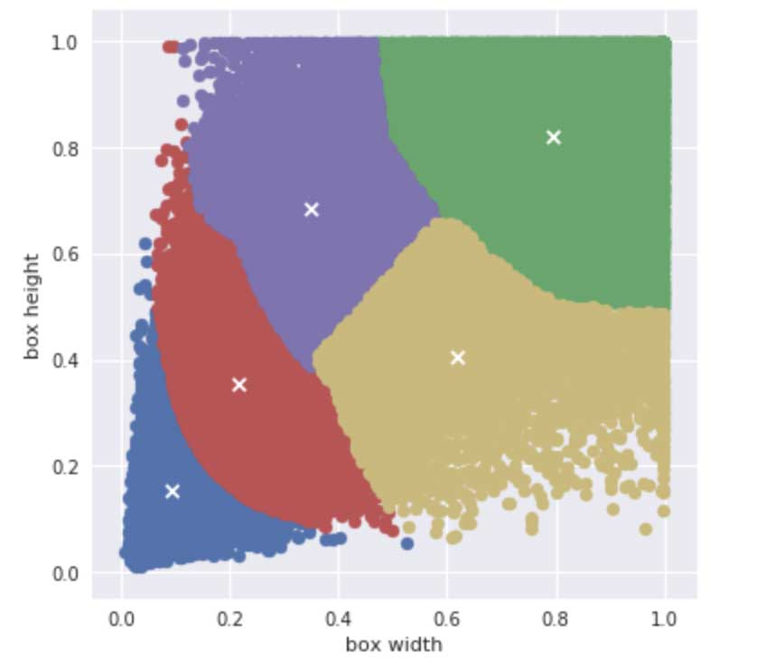
These clusters represent five “averages” of the different object shapes that are present in this dataset. You can see that k-means found it necessary to group very small objects together in the blue cluster, slightly larger objects in the red cluster, and very large objects in green. It decided to split medium objects into two groups: one where the bounding boxes are wider than tall (yellow), and one that’s taller than wide (purple).
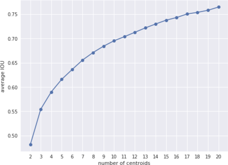
But is 5 anchors the optimal choice? We can run k-means several times on a different number of clusters, and compute the average IOU between the ground-truth boxes and the anchor boxes they are closest to. Not surprisingly, using more centroids (a larger value of k) gives a higher average IOU, but it also means we need more detectors in each grid cell and that makes the model run slower. For YOLO v2 they chose 5 anchors as a good trade-off between recall and model complexity.
SSD doesn’t use k-means to find the anchors. Instead it uses a mathematical formula to compute the anchor sizes. Therefore, SSD’s anchors are independent of the dataset (by the way, the SSD paper calls them “default boxes”). You’d think that anchors that are specific to the dataset would give better predictions but I’m not sure it really matters (the YOLO authors seem to think it does).
Another small difference: YOLO’s anchors are just a width and height, but SSD’s anchors also have an x,y-position. YOLO simply assumes that the anchor’s position is always in the center of the grid cell. (For SSD this is also the default thing to do.)
Thanks to anchors, the detectors don’t have to work very hard to make pretty good predictions already, because predicting all zeros simply outputs the anchor box, which will be reasonably close to the true object (on average). This makes training a lot easier! Without the anchors, each detector would have to learn from scratch what the different bounding box shapes look like… a much harder task.
Note: When I’m talking about YOLO in this article, I usually mean YOLO v2 or v3. If you’re reading papers or blog posts from around 2015-2016 and they mention YOLO, they’re often talking about YOLO v1, which is significantly different. Version 1 has a smaller grid (7×7 with only 2 detectors per cell), uses fully-connected layers instead of convolutional layers to predict the grid, and does not use anchors. That version of YOLO is obsolete now. The differences between v2 and v3 are much smaller. And with v3, YOLO has become quite similar to SSD in many ways.
What does the model actually predict?
Let’s look a bit closer at the output from the example model. Since it is just a convolutional neural network, a forward pass looks like this:
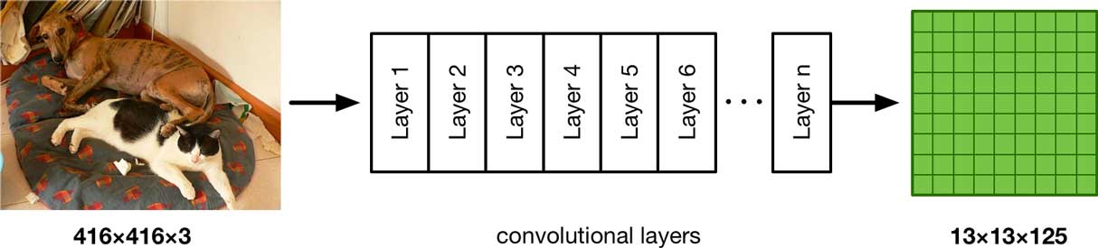
You input a 416×416-pixel RGB image, the convolutional layers apply all kinds of transformations on the image’s pixels, and the output is a 13×13×125 feature map. Because this is a regression output, no activation function is applied to the final layer. The output is just 21,125 real numbers, and we have to turn these numbers into bounding boxes somehow.
It takes 4 numbers to describe the coordinates of a bounding box. There are two common ways to do this: either as xmin, ymin, xmax, ymax to describe the edges of the box, or using center x, center y, width, height. Either method is fine, but we’ll use the latter (knowing where the center of the box is makes it easier to match the box to a grid cell).
What the model predicts for each bounding box is not their absolute coordinates in the image but four “delta” values, or offsets:
delta_x,delta_y: the center of the box inside the grid celldelta_w,delta_h: scaling factors for the width and height of the anchor box
Each detector makes a prediction relative to its anchor box. The anchor box should already be a pretty good approximation of the actual object size (which is why we’re using them) but it won’t be exact. This is why we predict a scaling factor that says how much larger or smaller the box is than the anchor, as well as a position offset that says how far off the predicted box is from this grid center.
To get the actual width and height of the bounding box in pixel coordinates, we do:
box_w[i, j, b] = anchor_w[b] * exp(delta_w[i, j, b]) * 32
box_h[i, j, b] = anchor_h[b] * exp(delta_h[i, j, b]) * 32
where i and j are the row and column in the grid (0 – 12) and b is the detector index (0 – 4).
It’s OK for the predicted box to be wider and/or taller than the original image, but it does not make sense for the box to have a negative width or height. That’s why we take the exponent of the predicted number.
If the predicted delta_w is smaller than 0, exp(delta_w) is a number between 0 and 1, making the box smaller than the anchor box. If delta_w is greater than 0, then exp(delta_w) a number > 1 which makes the box wider. And if delta_w is exactly 0, then exp(0) = 1 and the predicted box is exactly the same width as the anchor box.
By the way, we multiply by 32 because the anchor coordinates are in the 13×13 grid, each grid cell covers 32 pixels in the 416×416 input image.
Note: Interestingly enough, in the loss function we’ll actually use the inverse versions of the above formulas. Instead of doing exp() on the predicted values, we’ll take the log() of the ground-truth values. More about this below.
To get the center x,y position of the predicted box in pixel coordinates, we do:
box_x[i, j, b] = (i + sigmoid(delta_x[i, j, b])) * 32
box_y[i, j, b] = (j + sigmoid(delta_y[i, j, b])) * 32
A key feature of YOLO is that it encourages a detector to predict a bounding box only if it finds an object whose center lies inside the detector’s grid cell. This helps to avoid spurious detections, so that multiple neighboring grid cells don’t all find the same object.
To enforce this, delta_x and delta_y must be restricted to a number between 0 and 1 that is a relative position inside the grid cell. That’s what the sigmoid function is for.
Then we add the grid cell coordinates i and j (both 0 – 12) and multiply by the number of pixels per grid cell (32). Now box_x and box_y are the center of the predicted bounding box in the original 416×416 image space.
SSD does this slightly differently:
box_x[i, j, b] = (anchor_x[b] + delta_x[i, j, b]*anchor_w[b]) * image_w
box_y[i, j, b] = (anchor_y[b] + delta_y[i, j, b]*anchor_h[b]) * image_h
The predicted delta values here are actually multiples of the anchor box width or height, and there is no sigmoid activation. That means the center of the object can actually lie outside the grid cell with SSD.
Also note that with SSD the predicted coordinates are relative to the anchor box center rather than the center of the grid cell. In practice the anchor box’s center will line up exactly with the grid cell’s center, but they use different coordinate systems. SSD’s anchor coordinates are in the range [0, 1] to make them independent of the grid size. (This is done because SSD uses multiple grids of different sizes.)
As you can see, even though YOLO and SSD generally work in the same way, they are different when you start looking at the small details.
Besides coordinates, the model also predicts a confidence score for the bounding box. Because we want this to be a number between 0 and 1, we use the standard trick and stick it through a sigmoid:
confidence[i, j, b] = sigmoid(predicted_confidence[i, j, b])
Recall that our example model always predicts 845 bounding boxes, no more, no less. But typically there will be only a few real objects in the image. During training we encourage only a single detector to make a prediction for each ground-truth, so there will be only a few predictions with a high confidence score. The predictions from the detectors that did not find an object — by far the most of them — should have a very low confidence score.
And finally, we predict the class probabilities. In the case of the Pasval VOC dataset this is a vector of 20 numbers for each bounding box. As usual we apply a softmax make it a nice probability distribution:
classes[i, j, b] = softmax(predicted_classes[i, j, b])
Instead of a softmax you can also use a sigmoid activation. This makes it into a multi-label classifier, in which case each predicted bounding box can actually have multiple classes at the same time. (This is what SSD and YOLO v3 do.)
Note that SSD does not use this kind of confidence score. Instead, it adds a special class — “background” — to the classifier. If this background class is predicted, the detector did not find an object. This is the same thing as YOLO giving out a low confidence score.
Since we have many more predictions that we need, and most will be no good, we’ll now filter out the predictions with very low scores. In the case of YOLO, we do that by combining the confidence score for the box, which says “how likely is it that this box contains an object”, with the largest class probability, which says “how likely is it that this box contains an object of this class”.
confidence_in_class[i, j, b] = classes[i, j, b].max() * confidence[i, j, b]
A low confidence score means the model isn’t sure that this box really contains an object; a low class probability means the model isn’t certain what kind of object is in this box. Both scores need to be high for the prediction to be taken seriously.
Since most boxes will not contain any objects, we can now ignore all boxes whose confidence_in_class is below a certain threshold (such as 0.3), and then perform non-maximum suppression on the remaining boxes to get rid of duplicates. We typically end up with anywhere between 1 and about 10 predictions.
It is convolutional, baby!
Having a grid of detectors is actually a natural fit for using a convolutional neural network.
The 13×13 grid is the output of a convolutional layer. As you know, a convolution is a small window (or kernel) that slides over an input image. The weights for this kernel are the same at every input position. Our example model’s last layer has 125 of these kernels.

Why 125? There are 5 detectors and each detector has 25 convolution kernels. Each of these 25 kernels predicts one aspect of that detector’s bounding box: x, y, width, height, confidence score, the 20 class probabilities.
Note: In general, if your dataset has K classes and your model has B detectors, then the grid needs to have B × (4 + 1 + K) output channels.
These 125 kernels slide over each position in the 13×13 feature map, and at each position they make a prediction. We then interpret these 125 numbers as making up 5 predicted bounding boxes and their class scores for that grid position (this is the job of the loss function, more about that below).
Initially, the 125 numbers that get predicted at every grid position will be totally random and meaningless, but as training progresses the loss function will guide the model to learn to make more meaningful predictions.
Now, even though I keep saying there are 5 detectors in each grid cell, for 845 detectors overall, the model really only learns five detectors in total — not five unique detectors per grid cell. This is because the weights of the convolution layer are the same at each position and are therefore shared between the grid cells.
The model really learns one detector for every anchor. It slides these detectors across the image to get 845 predictions, 5 for each position on the grid. So even though we only have 5 unique detectors in total, thanks to the convolution these detectors are independent of where they are in the image and therefore can detect objects regardless of where they are located.
It’s the combination of the input pixels at a given location, with the weights that were learned for that detector / convolution kernel, that determine the final bounding box prediction at that position.
This also explains why model always predicts where the bounding box is relative to the center of the grid cell. Due to the convolutional nature of this model, it cannot predict absolute coordinates. Since the convolution kernels slide across the image, their predictions are always relative to their current position in the feature map.
YOLO versus SSD
The above description of how a one-stage object detector works applies to pretty much all of them. There may be small differences in exactly how the output is interpreted (sigmoid over the class probabilities instead of a softmax, for example) but the general idea is the same.
However, there are some interesting architectural differences between the various versions of YOLO and SSD.
Here is a sketch of the different architectures of YOLO v2 & v3, and SSD:
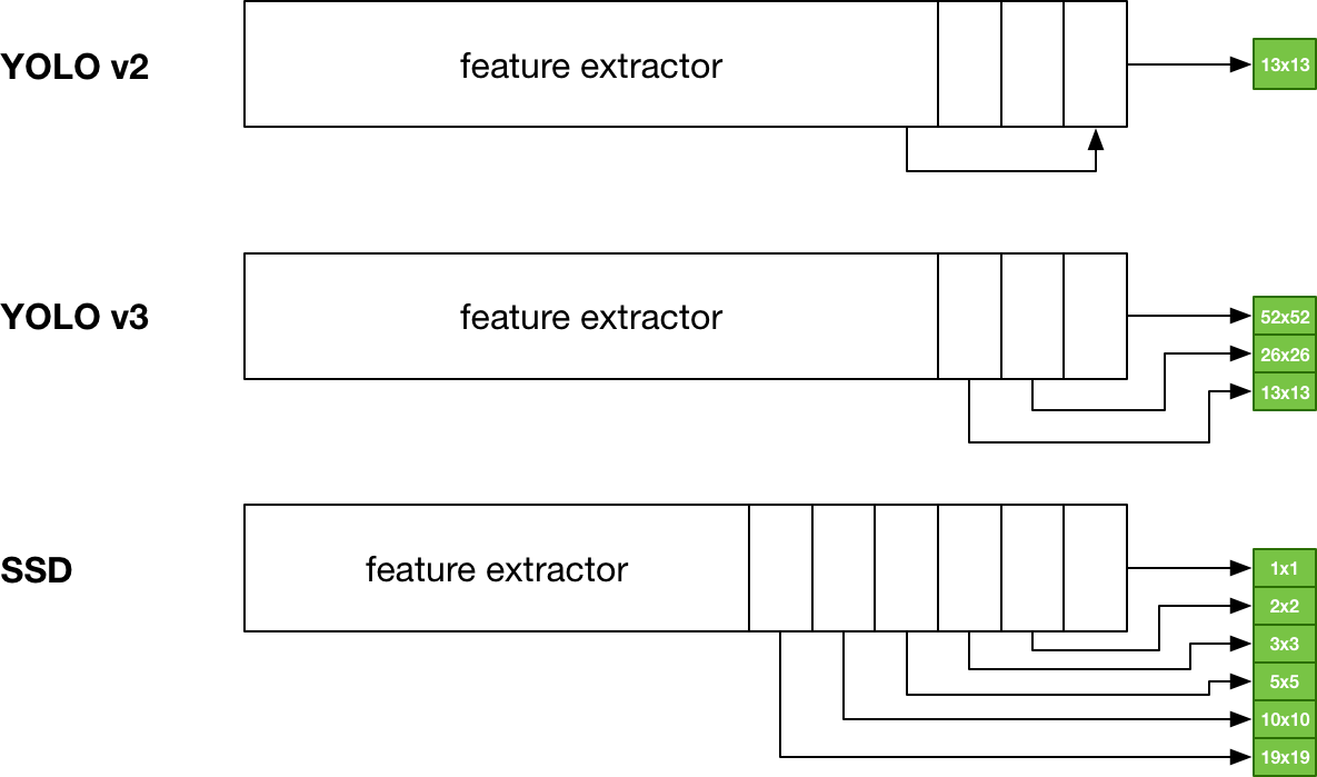
As you can see, at a high level YOLO v3 and SSD are quite similar, although they arrive at their final grid sizes through different methods (YOLO uses upsampling, SSD downsampling).
Where YOLO v2 (and our example model) only has a single 13×13 output grid, SSD has several grids of different sizes. The MobileNet+SSD version has 6 grids with sizes 19×19, 10×10, 5×5, 3×3, 2×2, and 1×1.
So the SSD grids range from very fine to very coarse. It does this to get more accurate predictions over a wider variety of object scales.
The fine 19×19 grid, whose grid cells are very close together, is responsible for the smallest objects. The 1×1 grid produced by the last layer is responsible for reacting to large objects which take up essentially the entire image. The grids from the other layers cover object sizes in between.
YOLO v2 tries to do something similar with its skip connection but this appears to be less effective. YOLO v3 is more like SSD in that it predicts bounding boxes using 3 grids that have different scales.
Like YOLO, each SSD grid cell makes multiple predictions. The number of detectors per grid cell varies: on the larger, more fine-grained feature maps SSD has 3 or 4 detectors per grid cell, on the smaller grids it has 6 detectors per cell. (YOLO v3 uses 3 detectors per grid cell at each scale.)
The coordinate predictions are relative to anchors as well — called “default boxes” in the SSD paper — but one difference is that SSD’s predicted center coordinates can go outside their grid cells. The anchor box is centered on the cell but SSD does not apply a sigmoid to the predicted x,y offset. So in theory a box in the bottom-right corner of the model could predict a bounding box with its center all the way over in the top-left corner of the image (but this probably won’t happen in practice).
Unlike YOLO, there is no confidence score. Each prediction consists of only the 4 bounding box coordinates and the class probabilities. YOLO uses the confidence score to indicate the chances of this prediction being of an actual object. SSD solves this differently by having a special “background” class: if the class prediction is for this background class, then it means there is no object found for this detector. This is the same thing as having a low confidence score in YOLO.
SSD’s anchors are a little different from YOLO’s. Because YOLO has to make all its predictions from a single grid, the anchors it uses range from small (about the size of a single grid cell) to large (about the size of the full image).
SSD is more conservative. The anchor boxes used on the 19×19 grid are smaller than those on the 10×10 grid, which are smaller than those in the 5×5 grid, and so on. Unlike YOLO, SSD does not use the anchors to make the detectors specialize on object size, it uses the different grids for that.
The SSD anchors are used mostly to make the detectors specialize on different possible aspect ratios of the objects’ shapes, not so much their sizes. As mentioned before, SSD’s anchors are computed using a simple formula while YOLO’s anchors are found by running k-means clustering on the training data.
Since SSD uses between 3 and 6 anchors and it has six grids instead of one, it actually uses more like 32 unique detectors in total (this number changes a bit depending on the exact model architecture you’re using).
Because SSD has more grids and detectors, it also outputs many more predictions. YOLO produces 845 predictions versus 1917 for MobileNet-SSD. A larger version, SSD512, even outputs 24,564 predictions! The advantage is that you’re more likely to find all objects in the image. The disadvantage is that you end up having to do more post-processing to figure out which predictions you want to keep.
Because of these differences, the way ground-truth bounding boxes are matched to detectors is a bit different between SSD and YOLO. The loss functions are slightly different as well. But we’ll cover that when we get to training.
Note: There is also a variant called SSDLite, which is the same as SSD but implemented with depthwise-separable convolutions rather than regular convolution layers. Thanks to this, it’s much faster than regular SSD and perfectly suited for use on mobile devices. Check out my Metal-based implementation of MobileNetV2+SSDLite here
OK, that’s enough theory about how these models make their predictions. Let’s now look at the kind of data we need to train an object detection model.
The data
There are several popular datasets for training object detection models — Pascal VOC, COCO, KITTI to name the big ones. Let’s look at Pascal VOC because it’s an important benchmark and it’s what’s used in the YOLO papers.
The VOC dataset consists of images plus annotations for different tasks. We’re only interested in the object detection task, so we’ll only look at images with object annotations. There are 20 object classes:
aeroplane    bicycle  bird   boat       bottle
bus          car      cat    chair      cow
diningtable  dog      horse  motorbike  person
pottedplant  sheep    sofa   train      tvmonitor
The VOC dataset comes with a suggested train/validation split that is roughly 50⁄50. The dataset isn’t very big so it does seem a little silly to use 50% of the data just for validation purposes. Because of this it’s typical to combine the train and validation sets into one big training set, “trainval” (16,551 images total), and randomly pick 10% or so of those images to be used for validation.
It’s possible to test your model on the 2007 test set since the answers are available. There is also a 2012 test set, but the answers to that are secret. (For submissions on the 2012 test set it’s also customary to include the 2007 test set in the training data. The more data, the merrier.)
Note: Even though the Pascal VOC competition is no longer active, you can still submit predictions to see how well your model scores on the leaderboard.
The combined 2007+2012 training set has 8218 images with object annotations, the validation set has 8333 images, and the 2007 test set has 4952 images. That’s a lot less than ImageNet’s 1.3 million images, and so it’s a good idea to use some kind of transfer learning instead of training the model from scratch. That’s why we start with a feature extractor that has been pre-trained on ImageNet.
Annotations
The annotations describe what is in the image. In order words, the annotations provide the targets we need for training.
The annotations are in XML format, one per training image. The annotation file contains one or more <object> sections, with the name of the class, a bounding box given as xmin, xmax, ymin, ymax, and a few other attributes for each ground-truth object.
If an object is marked as difficult, we will ignore it. These are often objects that are very small. Such objects are also ignored by the official evaluation metric for the VOC challenge.
Here is an example annotations file, VOC2007/Annotations/003585.xml:
<annotation>
    <folder>VOC2007</folder>
    <filename>003585.jpg</filename>
    <source>
        <database>The VOC2007 Database</database>
        <annotation>PASCAL VOC2007</annotation>
        <image>flickr</image>
        <flickrid>304100796</flickrid>
    </source>
    <owner>
        <flickrid>Huw Lambert</flickrid>
        <name>huw lambert</name>
    </owner>
    <size>
        <width>333</width>
        <height>500</height>
        <depth>3</depth>
    </size>
    <object>
        <name>person</name>
        <truncated>0</truncated>
        <difficult>0</difficult>
        <bndbox>
            <xmin>138</xmin>
            <ymin>183</ymin>
            <xmax>259</xmax>
            <ymax>411</ymax>
        </bndbox>
    </object>
    <object>
        <name>motorbike</name>
        <truncated>0</truncated>
        <difficult>0</difficult>
        <bndbox>
            <xmin>89</xmin>
            <ymin>244</ymin>
            <xmax>291</xmax>
            <ymax>425</ymax>
        </bndbox>
    </object>
</annotation>
This image is 333×500 pixels and has two objects: a person and a motorbike. Neither object is supposed to be difficult or truncated (partially outside the image). Like so many deep learning images, the original photo comes from Flickr.
Note: The Pascal VOC coordinates start counting at 1, not 0. This is probably because they used MATLAB which starts indexing at 1, like mathematicians do.
If we draw this training image and its bounding boxes, it looks like this:

For the combined 2007 and 2012 datasets, we have the following stats:
dataset   images    objects
------------------------------
train     8218      19910
val       8333      20148
test      4952      12032     (2007 only)
About half the images have just one object, the others have two or more. You can clearly see this in a histogram (this is for the training set):
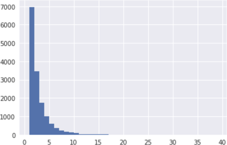
The maximum number of objects in one image is 39. The histograms for the validation and test sets are similar.
For fun, here is a histogram of the areas of all the bounding boxes in the training set, after normalizing the widths and heights to the range [0,1]:
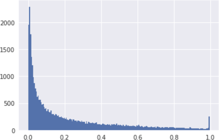
As you can see, many of the objects are relatively small. The peak at 1.0 is because there are quite a few objects that are larger than the image (for example, a human who’s only partially visible) and so the bounding box fills the entire image.
And here is another way to look at this data, a plot of the ground-truth bounding box widths versus their heights. The “slope” in this picture shows the aspect ratios of the boxes.
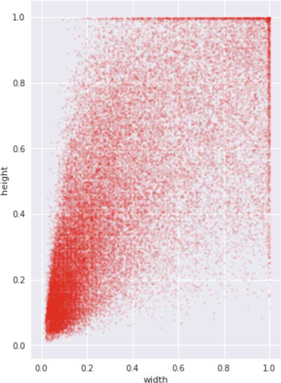
I find making these kinds of plots useful because it gives you some idea of what the data is like.
Data augmentation
Because the dataset is fairly small, it’s common to use a lot of data augmentation while training, such as random flips, random crops, color changes, etc.
It’s important to remember that whatever you do to the image must also be done to the bounding boxes! So if you flip the training image, you must also flip the coordinates for the ground-truth boxes.
YOLO does the following to load a training image:
- load the image without resizing
- pick a new width and height by randomly adding/subtracting 20% of the original size
- crop that part of the image, zero padding if the new image is larger on one or more sides than the original
- resize to 416×416, making it square
- randomly flip the image horizontally (with 50% probability)
- randomly distort the image’s hue, saturation, and exposure (brightness)
- also adjust the bounding box coordinates by shifting and scaling them to adjust for the cropping and resizing done earlier, and also for horizontal flipping
Rotation is also a common data augmentation technique but this gets tricky, as we’d also need to rotate the bounding boxes. So that’s typically not done.
The SSD paper also suggests the following augmentations:
- Randomly pick an image region so that the minimum IOU with the objects in the image is 0.1, 0.3, 0.5, 0.7, or 0.9. The smaller this IOU, the harder it will be for the model to detect the objects.
- Using a “zoom out” augmentation that effectively makes the image smaller, which creates extra training examples with small objects. This is useful for training the model to do better on small objects.
Doing random crops may cause objects to fall partially (or completely) outside of the cropped image. Because of this, we only want to keep the ground-truth boxes whose center is somewhere in this crop region, but not the boxes whose center now falls outside the visible image.
Beware of the aspect ratios!
Note: Feel free to skip this section. It deals with a issue that’s not important to get the big picture. But I haven’t really seen it addressed anywhere else, so I thought it was worth writing up.
We’re making our predictions on a square grid (13×13) and our input images are square too (416×416). But training images typically aren’t square and neither are the test images that we’ll be doing inference on. The images don’t even have all the same sizes.
Here is a visualization of all the aspect ratios of the images in the VOC training set:
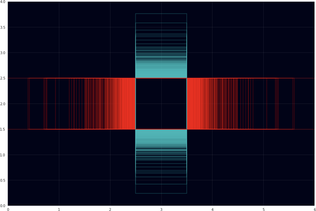
The red boxes have an aspect ratio that is wider than tall; the cyan boxes are taller than wide. There’s lots of weird aspect ratios but the most common ones are 1.333 (4:3), 1.5 (3:2), and 0.75 (3:4).
As you can see, some images are very wide. Here is an extreme example:

The neural network works on square images of size 416×416, so we have to fit the training image into that square. There are a few ways we can do this:
- non-uniformly resize to 416×416, this will squash the image
- resize the smallest side to 416, then take a 416×416 crop from the image
- resize the largest side to 416, padding the smaller side with zeros, and then take a crop
All are valid approaches but each has its own side effects.
When squashing the image, we change its aspect ratio to 1:1. If the original image was wider than tall, then all objects become more narrow than usual. If the original was taller than wide, then all objects become flatter.
By taking a crop the aspect ratio stays intact, but we may chop of important parts of the image, making it harder for the model to see an object for what it really is. The model may now need to predict a bounding box that is partially outside the image. (With option #3 it may make objects too small to be detected, especially if the aspect ratio is extreme.)
Why is this important?
Before training we will divide the bounding box’s xmin and xmax by the image width, and ymin and ymax by the image height, to normalize the coordinates so they are between 0 and 1. This is done to make training independent of the actual pixel size of each image.
But the input image isn’t usually square, so the x-coordinates get divided by a different number than the y-coordinates. These divisors will likely be different for each image, depending on the image’s dimensions and aspect ratio. And this affects how we should treat the bounding box coordinates and the anchors.
Squashing (option #1) is the easiest option, even though it temporarily messes up the image’s aspect ratio. If all images have a similar aspect ratio (which in VOC they don’t) or the aspect ratios are not too extreme, then the neural network should still work fine. Convnets seems to be fairly robust to “thickness” changes in objects.
With cropping (options #2 and #3), we should keep the aspect ratio in mind when normalizing the bounding box coordinates. It is now possible that the bounding box becomes larger than the input image, since we’re not looking at the entire image but only at a cropped portion. Since the objects may fall partially outside the image, so may the bounding boxes.
The downside of cropping is that we may lose important parts of the image — and that may be worse than squashing objects a little.
Whether you squash or crop also has an impact on how you compute the anchors from the dataset. The whole point behind using anchors is that these are like the most common object shapes in the dataset.
This remains true when cropping. Some of the anchors may now fall partially outside the image but at least their aspect ratios are truly representative of the objects in the training data.
With squashing, the computed anchors are not really representative of the true boxes since the different aspect ratios get ignored, as each training image gets squashed in a slightly different way. The anchors are now more of an average across many different image sizes that all get distorted in different ways.
The data augmentation also has an effect here. By taking randomly-sized crops of the image and then resizing to 416×416, those crops also mess up the aspect ratio (presumably on purpose).
Long short short: We’ll just stick with squashing the images and ignoring the aspect ratios of the bounding boxes, as it is simplest. It’s also what YOLO and SSD do.
One way to look at this, is that rather than trying to make the model respect the aspect ratios we’re actually trying to make it invariant to them. (If you know that you’ll always be working on input images of a fixed size, say 1280×720, then it may make more sense to use cropping.)
How do you train this thing?
We almost have all the pieces now to understand how this kind of object-detection model is trained.
The model makes predictions using a very straightforward convolutional neural network. We turn those predicted numbers into bounding boxes. The dataset contains the ground-truth boxes that say which objects are actually present in the training image, and so to train this kind of model we need to come up with a loss function that compares the predicted boxes to the ground-truths.
The problem is that the number of ground-truth boxes can vary between images, from zero to dozens. Those boxes may be all over the image, in any order. Some will overlap. During training, we must match each of our detectors with one of these ground-truth boxes, so that we can compute the regression loss for each predicted box.
If we naively perform this matching, for example by always assigning the first ground-truth object to the first detector, the second object to the second detector, and so on, or by randomly assigning the ground-truth objects to the detectors, then each detector will be trained to predict a wide variety of objects: some will be large, some will be small, some will be in one corner of the image, some will be in the opposite corner, some will be in the center, and so on.
This is the problem I mentioned way back at the beginning of this blog post, and why just adding a bunch of regression outputs to the model didn’t work. The solution was to use a grid with a fixed number of detectors, where each detector is only responsible for detecting objects that are located in that part of the image, and is only responsible for objects of a certain size.
Now the loss function needs to know which ground-truth object belongs to which detector in which grid cell, and likewise, which detectors do not have ground-truths associated with them. This is what we call “matching”.
Matching ground-truth boxes to detectors
How does this matching work? There are different strategies. The way YOLO does it is to make only one detector responsible for detecting a given object in the image.
First we find the grid cell that the center of the bounding box falls in. That grid cell will be responsible for this object. If any other grid cells also predict this object they will be penalized for it by the loss function.
The VOC annotations gives the bounding box coordinates as xmin, ymin, xmax, ymax. Since the model uses a grid and we decide which grid cell to use based on the center of the ground-truth box, it makes sense to convert the box coordinates to center x, center y, width, and height.
At this point we also want to normalize the box coordinates to the range [0, 1] so that they are independent of the size of the input image (since not all the training images have the same dimensions).
This is also where we apply data augmentation such as random horizontal flips and color changes (to both the image and its bounding boxes).
Note: Because of the data augmentation, which does random crops and flips, we have to re-compute the matching between ground-truth boxes and detectors in every epoch. This isn’t something we can pre-compute and cache, because the matches may change depending on the augmentation used for this particular image (which changes every epoch).
Just picking the cell is not enough. Each grid cell has multiple detectors and we only want one of these detectors to find the object, so we pick the detector whose anchor box best matches the object’s ground-truth box. This is done with the usual IOU metric.
This way, the smallest objects are assigned to detector 1 (which has the smallest anchor box), very large objects become the responsibility of detector 5 (which has the largest anchor box), and so on.
Only that particular detector in that cell is supposed to predict this object. This rule helps the different detectors to specialize in objects that have a shape and size that is similar to the anchor box. (Remember that the object doesn’t have to be the exact same size as the anchor, as the model predicts a position offset and size offset relative to the anchor box. The anchor box is just a hint.)
So for a given training image, some of the detectors will have an object associated with it, and all the other detectors won’t. If a training image has 3 unique objects in it, and thus 3 ground-truth boxes, then only 3 of the 845 detectors are supposed to make a prediction and the other 842 detectors are supposed to predict “no object” (which in terms of our model output is a bounding box with a very low confidence score, ideally 0%).

From now on, I’ll say positive example to mean a detector that has a ground-truth and negative example for a detector that does not have an object associated with it. A negative example is sometimes also called a “no object” or background.
Note: With classification we use the word “example” to refer to the training image as a whole but here it refers to an object inside an image, not to the image itself.
Since the output of the model is a 13×13×125 tensor, the target tensor that will be used by the loss function will also be 13×13×125. Again, that number 125 comes from: 5 detectors that each predict 20 probability values for the object’s class + 4 bounding box coordinates + 1 confidence score.
In the target tensor we only fill in the bounding boxes (and one-hot encoded class vector) for the detectors that are responsible for an object. We set the expected confidence score to 1 (since we’re 100% sure this is a real object).
For all other detectors — the ones with negative examples — the target tensor contains all zeros. The bounding box coordinates and class vector aren’t important here, since they will be ignored by the loss function, and the confidence score is 0 since we’re 100% sure there is no object here.
So when the training loop asks for a new batch of images and their targets, what it gets is a tensor of B×416×416×3 images and a tensor of B×13×13×125 numbers that represent the ground-truth boxes that we expect each of the detectors to predict. Most of the numbers in this target tensor will be 0 since most detectors will not be responsible for predicting an object.
There are some additional details to consider when matching. For example, what happens when there is more than one ground-truth box whose center happens to fall into the same cell? In practice this might not be a big problem, especially if the grid is fine enough, but still we need a way to handle such situations.
In theory if each box prefers a different detector based on the best IOU overlap — e.g. box A has the biggest IOU overlap with detector 2 and box B has the biggest overlap with detector 4 — then we could match both ground-truths to different detectors in this cell. However, that doesn’t avoid the problem of having two ground-truth boxes who want the same detector.
YOLO solves this by first randomly shuffling the ground-truths, and then it just picks the first one that matches the cell. So if a new ground-truth box is matched to a cell that already is responsible for another object, then we simply ignore this new box. Better luck next epoch!
This means that in YOLO at most one detector per cell is given an object — the other detectors in that cell are not supposed to detect anything (and are punished if they do).
Note that there are other possible matching strategies too. For example, SSD can match the same ground-truth box with multiple detectors: it first picks the detector with the best IOU, but then also chooses any (unassigned) detector whose anchor box has an IOU over 0.5 with this ground-truth. (I assume these detectors do not all have to be in the same cell, or even in the same grid, but the paper doesn’t say.)
This is supposed to make it easier for the model to learn because it won’t have to choose between which detector should predict an object — multiple detectors now have a shot at predicting this object.
Note: It may seem like some of these design choices are contradictory. YOLO assigns a ground-truth object to a single detector (and “no object” to the other detectors for this cell) in order to help the detectors specialize. But SSD says it’s OK for multiple detectors to predict the same object. Who is right? I don’t know. I’m not aware of any ablation studies between these particular choices. In the case of SSD, it’s probably OK since the detectors specialize on aspect ratio (shape) rather than size.
The loss function
As always, the loss function is what really tells the model what it should learn. For object detection, we want a loss function that encourages the model to predict correct bounding boxes and also the correct classes for these boxes. On the other hand, the model should not predict objects that aren’t there.
This is a complex task with multiple components. Therefore, our loss consists of several different terms (it’s a multi-task loss). Some of these terms are for regression, since they predict real-valued numbers; others are for classification.
For any given detector, there are two possible situations:
- This detector has no ground-truth associated with it. This is a negative example; it is not supposed to detect any objects (i.e. it should predict a bounding box with confidence score 0).
- This detector does have a ground-truth box. This is a positive example. The detector is responsible for detecting the object from the ground-truth box.
For detectors that are not supposed to detect an object, we will punish them when they predict a bounding box with a confidence score that is greater than 0.
Such detections are counted as false positives because there is no object present at this location in the image. Too many false positives reduces the precision of the model.
Conversely, if a detector does have a ground-truth box, we want to punish it:
- when the coordinates are wrong
- when the confidence score is too low
- when the class is wrong
Ideally, the detector predicts a box that exactly overlaps with the ground-truth box, has the same class label, and has a high confidence score.
When the confidence score is too low, the prediction counts as a false negative. The model didn’t find the object that is really there.
However, if the confidence score is good but the coordinates are wrong or the class is wrong, the prediction will be counted as a false positive. Even though the model claims it found an object, it’s the wrong one or it’s in the wrong place.
This means the same prediction can count both as a false negative (reducing the recall of the model) and a false positive (reducing the precision). Yikes. A prediction only counts as a true positive when all three aspects — coordinates, confidence, class — are correct.
Because so many different things can go wrong, the loss function consists of several parts that all measure a different kind of “wrongness” about the predictions the model made. These parts are added up to get the overall loss metric.
SSD, YOLO, SqueezeDet, DetectNet, and the other one-stage detector variants all use slightly different loss functions. Still, they tend to be composed of the same elements. Let’s look at the different parts!
Detectors with no ground-truth (negative examples)
This part of the loss function only involves the confidence score — since there is no ground-truth box here, we don’t have any coordinates or class label to compare the prediction to.
This loss term is only computed for the detectors that are not responsible for detecting an object. If such a detector does find an object, this is where it gets punished.
Recall that the confidence score represents whether the detector thinks there is an object with its center in this grid cell or not. The true confidence score in the target tensor is set to 0 for such a detector, since there is no object here. The predicted score also ought to be 0 — or close to it.
The loss for the confidence score needs to compare the predicted score with the true score somehow. In YOLO, it looks like this:
no_object_loss[i, j, b] = no_object_scale * (0 - sigmoid(pred_conf[i, j, b]))**2
where pred_conf[i, j, b] is the predicted confidence for cell i, j, and detector b inside that cell. Note that we use sigmoid() to restrict the predicted confidence to a number between 0 and 1 (making this into logistic regression).
To compute this loss term, we simply take the difference between the true value and the predicted value and then square it (the sum-squared error or SSE).
The no_object_scale is a hyperparameter. It’s typically 0.5, so that this part of the loss term doesn’t count as much as the other parts. Since the image will only have a handful of ground-truth boxes, most of the 845 detectors will only be punished by this “no object” loss and not any of the other loss terms I’ll show below.
Because we don’t want the model to learn only about “no objects”, this part of the loss shouldn’t become more important than the loss for the detectors that do have objects.
The above formula is for a single detector in a single cell. To find the aggregate no-object loss, we add up the no_object_loss for all cells i, j and all detectors b. For detectors that are responsible for finding an object, the no_object_loss is always 0. In SqueezeDet, the total no-object loss is also divided by the number of “no object” detectors to get the mean value but in YOLO we don’t do that.
Actually, YOLO has another trick up its sleeve. If the best IOU between a detector’s prediction and any of the ground-truth boxes in the image is greater than, say 60%, then no_object_loss[i, j, b] is set to 0.
In other words, if a detector wasn’t supposed to predict an object but it actually makes a really good prediction, then it’s probably a good idea to forgive it — and even encourage it to keep predicting objects. (In hindsight, we really should have made this detector responsible for that object.)
I’m not sure if this trick has any real effect on the final outcome, and it seems a bit hacky. But hey, where would machine learning be without hacks?
SSD does not have this no-object loss term. Instead, it adds a special background class to the possible classes. If that is the predicted class, then the output of that detector counts as “no object”.
Note: YOLO uses sum-squared error for all of these loss terms instead of the more common mean-squared error (MSE) for regression, or cross-entropy for classification.
Why sum-squared-error and not mean-squared-error? I’m not 100% sure but it might be because every image has a different number of objects in it (positive examples). If we were to take the mean, then an image with just 1 object in it may end up with the same loss as an image with 10 objects. With SSE, that latter image will have a loss that is roughly 10 times larger, which might be considered more fair.
It could also be because Darknet, the deep learning framework used for YOLO, is written in C and, unlike TensorFlow or PyTorch, does not have automatic differentiation. Using sum-squared-error gives a simpler gradient than MSE does (it is simply the ground-truth minus the prediction).
Detectors with a ground-truth (positive examples)
The previous section described what happens to detectors that are not responsible for finding objects. The only thing they can do wrong is find an object where there is none. Now we’ll look at the remaining detectors: the ones that are supposed to find objects.
These detectors can be wrong when they don’t find their object or when they misclassify the object. There are three separate loss terms that deal with this. We only compute these loss terms for detector b in grid cell i, j if that detector has a ground-truth box (i.e. if the confidence score in the target tensor is set to 1).
Confidence score
The loss term for the confidence score is:
object_loss[i, j, b] = object_scale * (1 - sigmoid(pred_conf[i, j, b]))**2
This is very similar to the no_object_loss, except the ground-truth here is 1, since we’re 100% sure there is an object here.
Actually, YOLO does something slightly more interesting:
object_loss[i, j, b] = object_scale *
         (IOU(truth_coords, pred_coords) - sigmoid(pred_conf[i, j, b]))**2
The predicted confidence score pred_conf[i, j, b] is supposed to represent the IOU between the predicted bounding box and the ground-truth box. Ideally this is 1 or 100%, for a perfect match. But instead of comparing the predicted score to this ideal number, YOLO looks at the actual IOU between the two boxes.
This makes sense: if the IOU is small then the confidence should be small, if the IOU is large then the confidence should be large too.
Unlike with the no-object loss, where we want the predicted confidence to be always 0, here we don’t just want the model to predict 100% confidence all the time. Instead, the model should learn to estimate how good its bounding box coordinates are. And that’s exactly what the IOU tells you.
As mentioned, SSD does not predict a confidence score and therefore does not have this loss term.
Class probabilities
Each detector also predicts the class of the object. This is independent of the bounding box coordinates. Essentially we train 5 separate classifiers that are all taught to look at objects of different sizes.
YOLO v1 and v2 used the following loss term for the predicted class probabilities:
class_loss[i, j, b] = class_scale * (true_class - softmax(pred_class))**2
Here, true_class is a one-hot encoded vector of 20 numbers (for Pascal VOC), and pred_class is the vector of predicted logits. Note that even though we apply a softmax to the predictions, this loss term does not use the cross-entropy. (I think maybe they used sum-squared-error because that makes this loss term easier to balance with the other loss terms. In fact, even the softmax is optional.)
YOLO v3 and SSD take a different approach. They don’t see this as a multi-class classification problem but as a multi-label problem. Hence they don’t use softmax (which always chooses a single label to be the winner) but a logistic sigmoid, which allows multiple labels to be chosen. They use a standard binary cross-entropy to compute this loss term.
Since SSD does not predict a confidence score, it has a special “background” class to serve this purpose. If a detector predicts background then that counts as the detector not finding an object (and we simply ignore those predictions). By the way, the SSD paper calls the loss term from this section the confidence loss, not the classification loss (just to be confusing).
Bounding box coordinates
And finally there is the loss term for the bounding box coordinates, also known as the localization loss. This is a simple regression loss between the four numbers that make up the bounding box.
coord_loss[i, j, b] = coord_scale * ((true_x[i, j, b] - pred_x[i, j, b])**2
                                   + (true_y[i, j, b] - pred_y[i, j, b])**2
                                   + (true_w[i, j, b] - pred_w[i, j, b])**2
                                   + (true_h[i, j, b] - pred_h[i, j, b])**2)
The scale factor coord_scale is used to make the loss from the bounding box coordinate predictions count more heavily than the other loss terms. A typical value for this hyperparameter is 5.
This loss term is simple enough but it’s important to realize what the true_* and pred_* values are in the above equation. Recall that all the way back in the section “What does the model actually predict?”, I gave the following code to find the actual bounding box coordinates:
box_x[i, j, b] = (i + sigmoid(pred_x[i, j, b])) * 32
box_y[i, j, b] = (j + sigmoid(pred_y[i, j, b])) * 32
box_w[i, j, b] = anchor_w[b] * exp(pred_w[i, j, b]) * 32
box_h[i, j, b] = anchor_h[b] * exp(pred_h[i, j, b]) * 32
We needed to do a little bit of post-processing to get valid coordinates out of the model’s predictions. The predicted x and y values had a sigmoid applied to them. And the predicted width and height are really scale factors that first needed to be exponentiated and then multiplied by the anchor’s width and height.
Because the model doesn’t directly predict valid coordinates, the ground-truth values used in the loss function are not supposed to be true coordinates either. Before we can use a ground-truth box in the loss function, we need to convert it:
true_x[i, j, b] = ground_truth.center_x - grid[i, j].center_x
true_y[i, j, b] = ground_truth.center_y - grid[i, j].center_y
true_w[i, j, b] = log(ground_truth.width / anchor_w[b])
true_h[i, j, b] = log(ground_truth.height / anchor_h[b])
Now true_x, true_y are relative to the grid cell, and true_w and true_h are proper scaling factors for the anchor’s dimensions. It’s important that we apply this inverse transformation when we fill in the target tensor, otherwise the loss function will be comparing apples and oranges.
SSD again uses a slightly different loss term. Its localization loss is known as the “Smooth L1” loss. Instead of simply taking the squared difference, this loss does something a bit more fancy:
difference = abs(true_x[i, j, b] - pred_x[i, j, b])
if difference < 1:
    coord_loss_x[i, j, b] = 0.5 * difference**2
else:
    coord_loss_x[i, j, b] = difference - 0.5
And so on for the other coordinates too. This loss is supposed to be less sensitive to outliers.
Ready to train!
And that’s it. Now all the pieces to train the model are complete. You have:
- the dataset (such as Pascal VOC) that provides the images and the annotations (the ground-truth boxes)
- a model that has many object detectors organized in a grid
- a matching strategy for putting the ground-truth boxes into this grid to create the target tensor
- and a loss function that compares the predictions with that target.
All you need to do now is let SGD loose on it!
By the way, given how I’ve just described the loss function it may seem like you would need to use a few nested loops to compute the loss, since detectors for positive examples use different loss terms than detectors for negative examples.
Perhaps something like this (in pseudo code):
for i in 0 to 12:
  for j in 0 to 12:
    for b in 0 to 4:
      gt = target[i, j, b]   # ground-truth
      pred = grid[i, j, b]   # prediction from model

      # is this detector responsible for an object?
      if gt.conf == 1:
        iou = IOU(gt.coords, pred.coords)
        object_loss[i, j, b] = (iou - sigmoid(pred.conf[i, j, b]))**2
        coord_loss[i, j, b] = sum((gt.coords - pred.coords)**2)
        class_loss[i, j, b] = cross_entropy(gt.class, pred.class)
      else:
        no_object_loss[i, j, b] = (0 - sigmoid(pred.conf[i, j, b]))**2
And then the combined loss is:
loss = no_object_scale * sum(no_object_loss) +
          object_scale * sum(object_loss) +
           coord_scale * sum(coord_loss) +
           class_scale * sum(class_loss)
But you can actually vectorize these loops so that the entire loss function can run on the GPU, as follows:
# the mask is 1 for detectors that have an object, 0 otherwise
mask = (target.conf == 1)

# compute IOUs between each detector's predicted box and
# the corresponding ground-truth box from the target tensor
ious = IOU(target.coords, grid.coords)

# compute the loss terms for the entire grid at once:
object_loss = sum(mask * (ious - sigmoid(grid.conf))**2)
coord_loss = sum(mask * (target.coords - grid.coords)**2)
class_loss = sum(mask * (target.class - softmax(grid.class))**2)
no_object_loss = sum((1 - mask) * (0 - sigmoid(grid.conf))**2)
Now we always compute all the loss terms for all the detectors, but we use a mask to throw away the results that we don’t want to count.
Even though what we do in the loss function is a lot more complicated than for image classification, it’s actually not too bad once you understand what all the separate parts are for. And since YOLO, SSD, and the other one-stage models all use slightly different variations of these loss terms, there seems to be a fair amount of leeway in how you choose them.
There are a few more tricks that are used to train these networks that are worth mentioning:
- Multi-scale training. In practice, an object detector will be used with images of (many) different sizes, which in turn contain objects of different sizes. One way to make the network predict well across a variety of input dimensions is to randomly choose a new input size every 10 batches. Instead of always training on 416×416 images, this randomly trains on images from 320×320 to 608×608.
- Warm-up training. YOLO adds a fake ground-truth box in the center of each cell during early training steps, and uses this to compute an additional coordinate loss. This is done to encourage predictions to start matching the anchors for the detectors.
- Hard negative mining. I’ve pointed out a few times now that most of the detectors will not be responsible for detecting any objects. This means there are many more negative examples than positive examples. YOLO deals with this by using a hyperparameter (
no_object_scale) but SSD uses hard negative mining. Instead of using all the negative examples in the loss, it only uses the ones that are the most wrong (the false positives with the highest confidence).
Even though the model might work just fine once it’s trained, sometimes you need these kinds of tricks to kick-start the model into learning anything.
How well does the model work?
To find out how well a classification model is doing, you can simply count the number of correct predictions on a test set and divide by the total test images to get the classification accuracy.
With object detection there are several things we can compute a score for:
- the classification accuracy of each detected object
- how much the predicted object overlaps the real object (IOU)
- whether the model actually finds all the objects in the image (known as “recall”)
None of these is sufficient by itself.
For example, the IOU lets us count a prediction as correct (a true positive or TP) if it overlaps the bounding box of a ground-truth by more than 50%, or as incorrect otherwise (a false positive or FP).
But this is not enough to understand how well your model is doing, since it does not tell you when the model misses objects — if there are ground-truth boxes that the model did not produce any predictions for (false negatives, or FN).
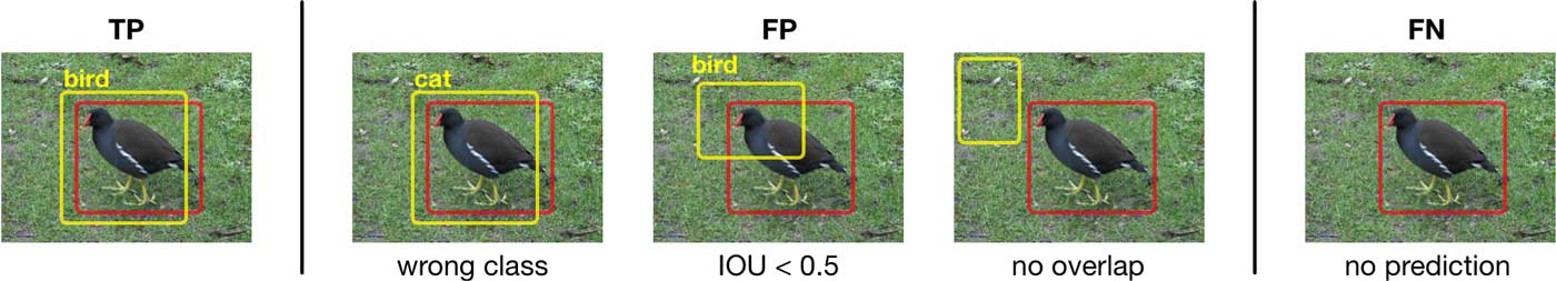
Note: There are no true negatives in object detection. A true negative is when a detector that is not responsible for predicting an object correctly predicts there is nothing there. That’s a good thing, but most of the time we don’t care about where the objects aren’t, only where they are. ;–)
To combine all these different facets into a single number, we typically use mean average precision or mAP. The higher the mAP, the better your model is. The current top scoring model on the Pascal VOC 2012 test set has mAP of 77.5% (refine_denseSSD from 14 May 2018). For comparison, YOLO v2 scores 48.8% and SSD scores 64% (this is likely the big version of SSD, not the fast mobile one).
There are a few different ways to compute the mAP, depending on the dataset you’re using. Since I’ve been talking about Pascal VOC all this time, let’s examine their method.
Computing the mAP
For the Pascal VOC mAP, first we compute the average precision (or AP) for each of the 20 classes separately, then we take the mean over these 20 numbers to get the final mAP score. So the mAP score is the average of an average.
The term precision in machine learning means something very specific, it is the number of true positives divided by the total number of detections:
precision = TP / (TP + FP)
In our case, a false positive is an object that was detected but does not actually exist in the image. This happens when a predicted bounding box is too different from any ground-truth box in the image, or when the predicted class is not the same.
Note: At this point, it doesn’t matter what detector the prediction came from. When evaluating the model we’re not assigning detectors to be responsible for specific objects — that only happens during training. Here, we’re just comparing the predicted bounding boxes to the ground-truths to see how many objects we’ve found.
Another metric that is often used together with precision is recall, also known as the true positive rate or the sensitivity:
recall = TP / (TP + FN)
The only difference in these formulas is that precision uses the number of false positives in the denominator while recall uses the number of false negatives. A false negative happens when no prediction is made for an object, or when the confidence score is too low (which really means the same as “no prediction”).
Informally, the precision measures: of how all the objects you predicted were a “cat”, how many really are cats? (Here, FP is how many predicted cats were not really cats — or objects at all.)
The recall measures how many of the cats that were in the image you actually found (FN is how many cats you missed).
For example, if you predicted there were three cats in an image but one of them is really a dog and the other is not an object at all, the precision for the cat class is 1⁄3 = 0.33. (One correct out of three predictions.)
If there were actually 4 cats in the image, the recall for cat is 1⁄4 = 0.25 because you only found one of them. And if there was only one dog in that image, precision and recall for dog are both 0 since you mistakenly thought it was a cat.
Here is how to compute the number of TP and FP, in pseudocode:
sort the predictions by confidence score (high to low)

for each prediction:
    true_boxes = get the annotations with same class as the prediction
                     and that are not marked as "difficult"

    find IOUs between true_boxes and prediction
    choose ground-truth box with biggest IOU overlap

    if biggest IOU > threshold (which is 0.5 for Pascal VOC):
        if we do not already have a detection for this ground-truth box:
            TP += 1
        else:
            FP += 1
    else:
        FP += 1
A prediction counts as a true positive if it has the same class as a ground-truth object and their bounding boxes overlap by more than 50%. If the overlap is less than 50%, the prediction counts as a false positive.
According to the Pascal VOC rules, if two or more predictions have an IOU greater than 50% with the same ground-truth bounding box, we must choose only one as the correct prediction. The other detections will be counted as false positives. This is done to encourage models to predict only one box per object. (We choose the prediction with the highest confidence score as the correct one, not necessarily the one with the largest IOU.)
Since multiple predictions for the same object are penalized, it’s smart to first apply non-maximum suppression (NMS) to get rid of overlapping predictions as much as possible.
It’s also a good idea to throw away predictions with a very low confidence score (anything with a score below 0.3, for example). These would otherwise count as false positives. With a model such as YOLO, which always produces 845 predictions, or SSD with 1917 predictions, there will always be many more predictions than real objects (the vast majority of images only contains 1 to 3 real objects).
We have not counted false negatives at this point yet, but we don’t really need to. The denominator for recall is TP + FN, which is actually the same as the number of ground-truth boxes in the image (for the particular class we’re looking at).
Now we have all we need to compute the precision and recall. However, a single precision and recall score doesn’t really say much about the model, and so we’ll compute a whole range of precision, recall pairs and plot the result as a curve called… wait for it… the precision-recall curve.
We’ll create such a curve for each of the 20 classes. The average precision (AP) for a class is then the area under its curve.
The precision-recall curve
This is the precision-recall curve for the class “dog” of one of my experimental models:
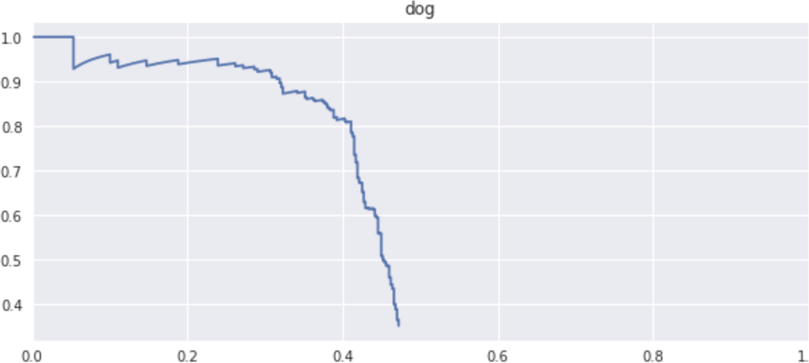
On the x-axis is the recall, going from 0 (no ground-truth objects found) to 1 (all objects found). On the y-axis is the precision. Note that precision is given as a function of recall, which is why the area under the curve is the average of the precision for this class. That’s where the metric “mean average precision” gets its name: we want to know what the precision is for different values of recall.
Note that the above precision-recall curve isn’t really that great yet. The area under the curve — the average precision for class “dog” — is only 0.42. Hey, like I said, it’s from an experimental model. ;–)
How to interpret this curve?
A precision-recall curve is always created by computing the precision and recall scores at different thresholds. For a binary classifier this is the threshold after which we conclude that a prediction is positive. In the case of an object detection model, the threshold we’re varying is the confidence score of the predicted boxes.
First we compute precision and recall for the first prediction (highest threshold), then we compute precision and recall for the first and second predictions (slightly lower threshold), then for the top three predictions (even lower threshold), and so on until we get to the end of the list where we compute precision and recall over all predictions (lowest threshold).
Each of these precision/recall values is a point on the curve (an operating point), with recall on the x-axis and precision on the y-axis.
At high thresholds, recall will be low since only a few predictions are included and so there will be many false negatives. You can see this on the left-hand side of the curve: precision is high at 100% but that’s because we only include the predictions we’re extremely sure about. But the recall is very low here, as we’re leaving out a lot of objects.
As the threshold decreases and we’re including more objects in the result, recall increases. Precision can go up and down, although it tends to become lower since now more false positives are found.
At the lowest threshold, recall is at its maximum, since we’re now looking at all the predictions made by the model. For my experimental model the recall for dog tops out at 42%, so even at this lowest threshold it only finds 4 out of every 10 dogs on average. There’s room for improvement here!
I hope this makes it clear there’s always a trade-off between false positives and false negatives predicted by the model. The reason we’re using a precision-recall curve is to measure that trade-off, and to find a good threshold for the confidence score.
Choosing a high threshold means we keep fewer predictions, and therefore we’ll have fewer false positives (we make fewer mistakes) but we’ll also have more false negatives (we miss more objects).
The lower the threshold, the more predictions we include but they’ll usually be of lower quality.
Ideally, the precision is high for every recall. Taking the average of the precision over all possible recall values gives us a useful summary of how well the model works for detecting objects of this particular class.
Once we have the precision and recall for all different threshold values, we can compute the average precision (AP) by finding the area under this curve. There are actually two different methods for this in Pascal VOC: the 2007 test set used an approximate method; the 2012 version is more exact (uses integration) and tends to give a slightly lower score.
The final mAP score is simply the average over the average precisions for the 20 classes.
Naturally, a higher score is better. But that doesn’t mean the mAP is all that matters. YOLO scores lower than some of its competition, but it’s also faster. Especially for use on mobile devices, we want to use models that have a good trade-off between speed and accuracy.
Fast object detection on iOS
I have recently written a library for iOS and macOS that contains fast Metal-based implementations of MobileNet V1 and V2, with support for SSD and SSDLite.
I’ve found that SSD — and especially SSDLite — works much faster than YOLO v2 on mobile and has similar accuracy. You might expect YOLO to be faster since it only has a single grid while SSD uses multiple grids, but unfortunately YOLO’s feature extractor is not optimized for mobile.
If you’re looking for a fast object detector to add into your apps, MobileNetV2 + SSDLite is a good place to get started. Click here to learn more
First published on Saturday, 9 June 2018.
If you liked this post, say hi on Twitter @mhollemans or LinkedIn.
Find the source code on my GitHub.
 New e-book: Code Your Own Synth Plug-Ins With C++ and JUCE
Interested in how computers make sound? Learn the fundamentals of audio programming by building a fully-featured software synthesizer plug-in, with every step explained in detail. Not too much math, lots of in-depth information! Get the book at Leanpub.com