
A little less than a year ago I wrote about MobileNets, a neural network architecture that runs very efficiently on mobile devices. Since then I’ve used MobileNet V1 with great success in a number of client projects, either as a basic image classifier or as a feature extractor that is part of a larger neural network.
Recently researchers at Google announced MobileNet version 2. This is mostly a refinement of V1 that makes it even more efficient and powerful. Naturally, I made an implementation using Metal Performance Shaders and I can confirm it lives up to the promise.
In this blog post I’ll explain what’s new in MobileNet V2.
Quick recap of version 1
The big idea behind MobileNet V1 is that convolutional layers, which are essential to computer vision tasks but are quite expensive to compute, can be replaced by so-called depthwise separable convolutions.
The job of the convolution layer is split into two subtasks: first there is a depthwise convolution layer that filters the input, followed by a 1×1 (or pointwise) convolution layer that combines these filtered values to create new features:
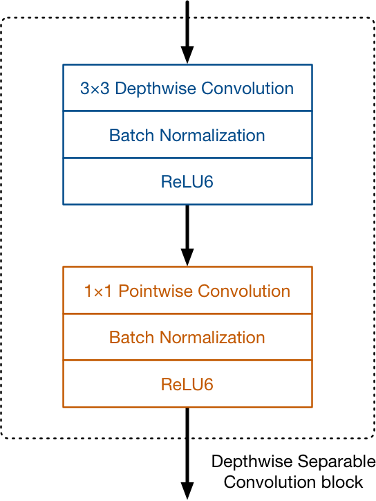
Together, the depthwise and pointwise convolutions form a “depthwise separable” convolution block. It does approximately the same thing as traditional convolution but is much faster.
The full architecture of MobileNet V1 consists of a regular 3×3 convolution as the very first layer, followed by 13 times the above building block.
There are no pooling layers in between these depthwise separable blocks. Instead, some of the depthwise layers have a stride of 2 to reduce the spatial dimensions of the data. When that happens, the corresponding pointwise layer also doubles the number of output channels. If the input image is 224×224×3 then the output of the network is a 7×7×1024 feature map.
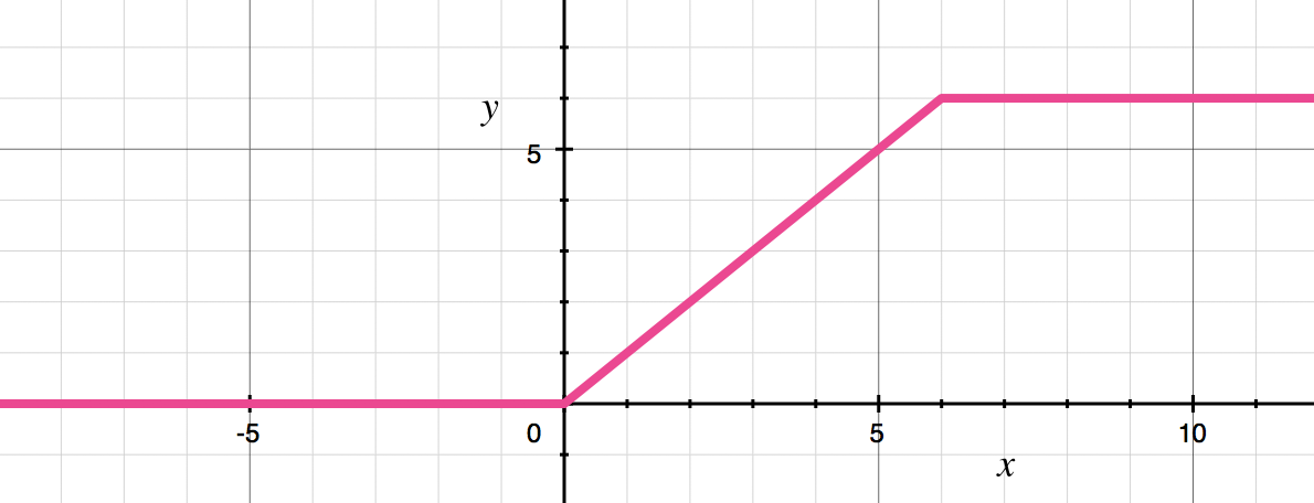
As is common in modern architectures, the convolution layers are followed by batch normalization. The activation function used by MobileNet is ReLU6. This is like the well-known ReLU but it prevents activations from becoming too big:
y = min(max(0, x), 6)
The authors of the MobileNet paper found that ReLU6 is more robust than regular ReLU when using low-precision computation. (I think “low-precision” here refers to fixed-point arithmetic and not so much the 16-bit floats used with Metal on iOS.)
It also makes the shape of the function look more like a sigmoid:
In a classifier based on MobileNet, there is typically a global average pooling layer at the very end, followed by a fully-connected classification layer or an equivalent 1×1 convolution, and a softmax.
There is actually more than one MobileNet. It was designed to be a family of neural network architectures. There are several hyperparameters that let you play with different architecture trade-offs.
The most important of these hyperparameters is the depth multiplier, confusingly also known as the “width multiplier”. This changes how many channels are in each layer. Using a depth multiplier of 0.5 will halve the number of channels used in each layer, which cuts down the number of computations by a factor of 4 and the number of learnable parameters by a factor 3. It is therefore much faster than the full model but also less accurate.
Thanks to the innovation of depthwise separable convolutions, MobileNet has to do about 9 times less work than comparable neural nets with the same accuracy. This type of layer works so well that I’ve been able to get models with 200+ layers to run in real-time, even on an iPhone 6s.
All right, so that’s all old news. For a more in-depth look, check out my previous blog post or the original paper.
The all new version 2
MobileNet V2 still uses depthwise separable convolutions, but its main building block now looks like this:
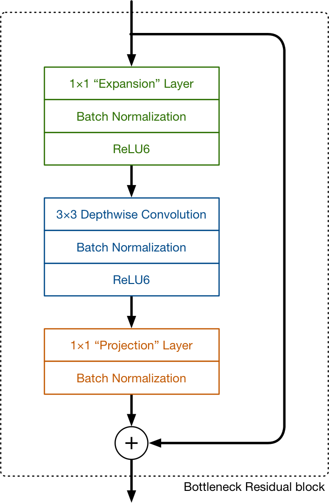
This time there are three convolutional layers in the block. The last two are the ones we already know: a depthwise convolution that filters the inputs, followed by a 1×1 pointwise convolution layer. However, this 1×1 layer now has a different job.
In V1 the pointwise convolution either kept the number of channels the same or doubled them. In V2 it does the opposite: it makes the number of channels smaller. This is why this layer is now known as the projection layer — it projects data with a high number of dimensions (channels) into a tensor with a much lower number of dimensions.
For example, the depthwise layer may work on a tensor with 144 channels, which the projection layer will then shrink down to only 24 channels. This kind of layer is also called a bottleneck layer because it reduces the amount of data that flows through the network. (This is where the “bottleneck residual block” gets its name from: the output of each block is a bottleneck.)
The first layer is the new kid in the block. This is also a 1×1 convolution. Its purpose is to expand the number of channels in the data before it goes into the depthwise convolution. Hence, this expansion layer always has more output channels than input channels — it pretty much does the opposite of the projection layer.
Exactly by how much the data gets expanded is given by the expansion factor. This is one of those hyperparameters for experimenting with different architecture tradeoffs. The default expansion factor is 6.
For example, if there is a tensor with 24 channels going into a block, the expansion layer first converts this into a new tensor with 24 * 6 = 144 channels. Next, the depthwise convolution applies its filters to that 144-channel tensor. And finally, the projection layer projects the 144 filtered channels back to a smaller number, say 24 again.

So the input and the output of the block are low-dimensional tensors, while the filtering step that happens inside block is done on a high-dimensional tensor.
The second new thing in MobileNet V2’s building block is the residual connection. This works just like in ResNet and exists to help with the flow of gradients through the network. (The residual connection is only used when the number of channels going into the block is the same as the number of channels coming out of it, which is not always the case as every few blocks the output channels are increased.)
As usual, each layer has batch normalization and the activation function is ReLU6. However, the output of the projection layer does not have an activation function applied to it. Since this layer produces low-dimensional data, the authors of the paper found that using a non-linearity after this layer actually destroyed useful information.
NOTE: The pre-trained models from tensorflow/models only use batch normalization after the depthwise convolution layer, the 1×1 convolutions use bias instead. I’m not sure why that is the case but in practice it doesn’t matter — for inference the batch norm operation gets folded into the convolution layer anyway.
The full MobileNet V2 architecture, then, consists of 17 of these building blocks in a row. This is followed by a regular 1×1 convolution, a global average pooling layer, and a classification layer. (Small detail: the very first block is slightly different, it uses a regular 3×3 convolution with 32 channels instead of the expansion layer.)
Motivation for these changes
Why did the authors of MobileNet V2 make these choices?
The idea behind V1 was to replace expensive convolutions with cheaper ones, even if it meant using more layers. That was a great success. The main changes in the V2 architecture are the residual connections and the expand/projection layers.
If we look at the data as it flows through the network, notice how the number of channels stays fairly small between the blocks:

As is usual for this kind of model, the number of channels is increased over time (and the spatial dimensions cut in half). But overall, the tensors remain relatively small, thanks to the bottleneck layers that make up the connections between the blocks. Compared to this, V1 lets its tensors become much larger (up to 7×7×1024).
Using low-dimension tensors is the key to reducing the number of computations. After all, the smaller the tensor, the fewer multiplications the convolutional layers have to do.
However… only using low-dimensional tensors doesn’t work very well. Applying a convolutional layer to filter a low-dimensional tensor won’t be able to extract a whole lot of information. So to filter the data we ideally want to work with large tensors. MobileNet V2’s block design gives us the best of both worlds.
Think of the low-dimensional data that flows between the blocks as being a compressed version of the real data. In order to run filters over this data, we need to uncompress it first. That’s what happens inside each block:
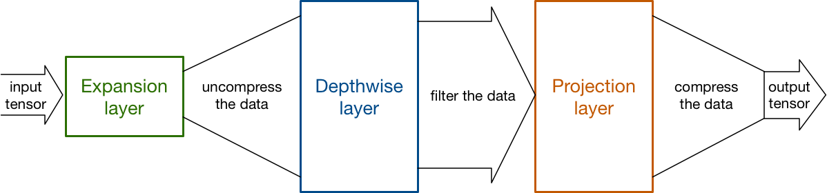
The expansion layer acts as an decompressor (like unzip) that first restores the data to its full form, then the depthwise layer performs whatever filtering is important at this stage of the network, and finally the projection layer compresses the data to make it small again.
The trick that makes this all work, of course, is that the expansions and projections are done using convolutional layers with learnable parameters, and so the model is able to learn how to best (de)compress the data at each stage in the network.
Battle of the versions
Let’s compare MobileNet V1 to V2, starting with the sizes of the models in terms of learned parameters and required amount of computation:
| Version | MACs (millions) | Parameters (millions) |
|---|---|---|
| MobileNet V1 | 569 | 4.24 |
| MobileNet V2 | 300 | 3.47 |
These numbers are taken from 1 and 2. They are for the model versions with a 1.0 depth multiplier. In this table, lower numbers are better.
“MACs” are multiply-accumulate operations. This measures how many calculations are needed to perform inference on a single 224×224 RGB image. (The larger the image, the more MACs are needed.)
From the number of MACs alone, V2 should be almost twice as fast as V1. However, it’s not just about the number of calculations. On mobile devices, memory access is much slower than computation. But here V2 has the advantage too: it only has 80% of the parameter count that V1 has.
NOTE: I’m not entirely sure how they counted these parameters. My Metal version of the V1 model has 4,254,889 parameters and the V2 model has 3,510,505, so that’s slightly more than what is reported above. It’s possible they’re not counting the batch normalization parameters as these typically get folded into a single set of biases for each layer.
I also measured the actual speed difference between the two models on a few devices, running inference on a sequence of 224×224 images. The following table shows the maximum FPS (frames-per-second) I was able to squeeze from these models:
| Version | iPhone 7 | iPhone X | iPad Pro 10.5 |
|---|---|---|---|
| MobileNet V1 | 118 | 162 | 204 |
| MobileNet V2 | 145 | 233 | 220 |
For optimal throughput I used a double-buffering approach where the next request is already being prepared (by the CPU) while the current one is still being processed (by the GPU). This way the CPU and GPU are never waiting for one another.
(Fun fact: for V2 it was actually worth doing triple buffering but for V1 that made no difference in speed. This shows that V2 is much more efficient.)
Having a fast model is great… but it’s only useful if it actually computes the right thing. So exactly how good are these models?
| Version | Top-1 Accuracy | Top-5 Accuracy |
|---|---|---|
| MobileNet V1 | 70.9 | 89.9 |
| MobileNet V2 | 71.8 | 91.0 |
The reported top-1 and top-5 accuracy are on the ImageNet classification dataset. (The source for these numbers claims they’re from the test set but looking at the code it appears to be the 50,000-image validation set.)
It can be a bit misleading to compare accuracy numbers between models, since you need to understand exactly how the model is evaluated. To get the above numbers, the central region of the image was cropped to an area containing 87.5% of the original image, and then that crop was resized to 224×224 pixels. Only a single crop was used per image.
NOTE: Naturally, I did verify that my Metal version of MobileNet V2 comes up with the same answers as the TensorFlow reference model, but I have not tried it on the ImageNet validation set yet. It will be interesting to see if the Metal version gets the same score. :–)
Conclusion: In all of these metrics, V2 scores better than V1. I’m especially pleased that it uses fewer parameters because that’s where most of the speed gains come from on mobile devices.
More than just classification
While the classification score on the ImageNet dataset is useful to know, in practice you’ll probably never use the pre-trained ImageNet classifier in your apps.
You’ll either re-train the classifier on your own dataset, or use the base network as a feature extractor for something like object detection (finding multiple objects in the same image) or image segmentation (making a class prediction for every pixel instead of a single prediction for the whole image) or some other exciting computer vision task.
Re: object detection, I’ve written about YOLO before. Since then, SSD (Single Shot Detector) has been making a name for itself. It uses many of the same ideas as YOLO but works even better — the main difference is that YOLO makes predictions for only a single feature map while SSD combines predictions across multiple feature maps at different sizes.
I’m currently writing a blog post that goes into detail on how these object detectors work and how to train one from scratch, but I just wanted to point out here that MobileNet and SSD make a great combination.
The problem with YOLO on mobile is that, while the actual detection portion of the neural network is simple and fast, the feature extractor (Darknet-19) uses regular convolutional layers. Running YOLO on an iPhone only gets you about 10 – 15 FPS. YOLO would be much faster if it was running on top of MobileNet instead of the Darknet feature extractor.
SSD is designed to be independent of the base network, and so it can run on top of pretty much anything, including MobileNet. Even better, MobileNet+SSD uses a variant called SSDLite that uses depthwise separable layers instead of regular convolutions for the object detection portion of the network. With SSDLite on top of MobileNet, you can easily get truly real-time results (i.e. 30 FPS or more).
How does this work? When doing classification, the last layers of the neural network look like this:
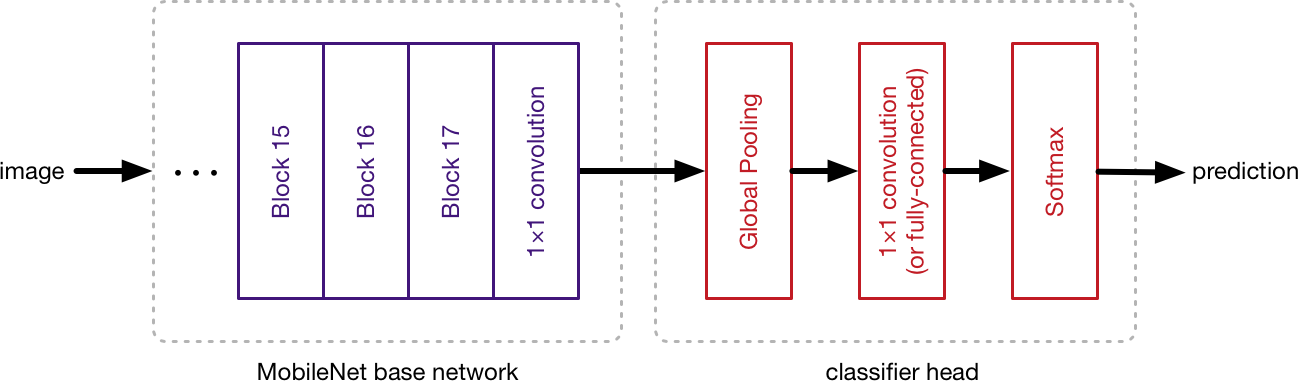
The output of the base network is typically a 7×7 pixel image. The classifier first uses a global pooling layer to reduce the size from 7×7 to 1×1 pixel — essentially taking an ensemble of 49 different predictors — followed by a classification layer and a softmax.
To use something like SSDLite with MobileNet, the last layers will look like this instead:
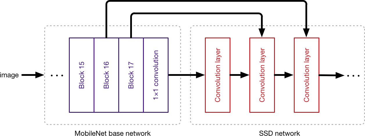
Not only do we take the output of the last base network layer but also the outputs of several previous layers, and we feed these outputs into the SSD layers. The job of the MobileNet layers is to convert the pixels from the input image into features that describe the contents of the image, and pass these along to the other layers. Hence, MobileNet is used here as a feature extractor for a second neural network.
In the case of classification, we’re interested in the features that describe high-level concepts, such as “there is a face” and “there is fur”, which the classifier layer then can use to draw a conclusion — “this image contains a cat”.
In the case of object detection with SSD, we want to know not just these high-level features but also lower-level ones, which is why we also read from the previous layers. Since object detection is more complicated than classification, SSD adds many additional convolutional layers on top of the base network. So it’s important to have a feature extractor that is fast — and that’s exactly what MobileNet V2 is.
The MobileNet V2 paper also shows that it’s possible to run an advanced semantic segmentation model such as DeepLabv3 on top of MobileNet-extracted features.
What next?
If you’re thinking of building a neural network for use on iOS devices — or even macOS — then using MobileNet as the base feature extractor for your model is a good idea, especially if you need to optimize for speed (and also battery usage).
Over the past year, I’ve helped clients build all kinds of exciting models on top of MobileNet V1 and I expect to be doing the same for V2, given that it’s faster, uses less memory, and is better at conserving battery power.
NOTE: Another option is SqueezeNet, which uses even fewer parameters than MobileNet, but it’s optimized mostly for low memory situations, not so much for speed. It also has lower accuracy. Recently a new version was announced, SqueezeNext, and I’m interested in comparing this to MobileNet V2, so I might write a future blog post about this.
How to get MobileNet V2. I have written a library for iOS and macOS that contains fast Metal-based implementations of MobileNet V1 and V2, as well as SSDLite and DeepLabv3+. This library makes it very easy to add MobileNet into your apps, either as a classifier, for object detection, or as a feature extractor that’s part of a custom model. Click here to learn more
First published on Sunday, 22 April 2018.
If you liked this post, say hi on Twitter @mhollemans or LinkedIn.
Find the source code on my GitHub.
 New e-book: Code Your Own Synth Plug-Ins With C++ and JUCE
Interested in how computers make sound? Learn the fundamentals of audio programming by building a fully-featured software synthesizer plug-in, with every step explained in detail. Not too much math, lots of in-depth information! Get the book at Leanpub.com