
Because I focus on deep learning on mobile, I’m naturally interested in finding ways to make deep neural networks faster and more energy efficient.
One way is to come up with smarter neural net designs. For example, MobileNet is 32× smaller and 10× faster than VGG16 but produces the same results.
Another method is to take an existing neural network and compress it, by removing connections between neurons that don’t really add much to the final result. That’s what I want to talk about in this blog post.
We’re going to take MobileNet-224 and make it 25% smaller. In other words, we’re going to reduce it from 4 million parameters to 3 million — without losing accuracy (well… only a little).
Can we do better?
Since MobileNet is 32 times smaller than VGG16, yet has the same accuracy, it must be more efficient at capturing knowledge than VGG is.
It’s indeed a known fact that VGG has way more connections than it needs in order to do its job. The Deep Compression paper by Han et al. shows that the size of VGG16 can be reduced by a factor 49 by pruning unimportant connections and it will still give the same answers.
The question is: does MobileNet have any connections it doesn’t really need? Even though this model is already quite small, can we make it even smaller — without making it worse?
When you compress a neural network, the tradeoff is network size vs. accuracy. In general, the smaller the network, the faster it runs (and the less battery power it uses) but the worse its predictions are. MobileNet scores better than SqueezeNet, for example, but is also 3.4 times larger.
Ideally, we want to find the smallest possible neural net that can most accurately represent the thing we want it to learn. This is an open problem in machine learning, and until there is a good theory of how to do this, we’re going to have to start with a larger network and lobotomize it.
For this project I used the pre-trained version of MobileNet that comes with Keras 2.0.7, running on TensorFlow 1.0.3. Evaluating this model on the ImageNet ILSVRC 2012 validation set gives the following scores:
Top-1 accuracy over 50000 images = 68.4%
Top-5 accuracy over 50000 images = 88.3%
This means it has guessed the correct answer 68.4% of the time, while 88.3% of the time the correct answer was among its five best guesses. We want the compressed model to get an accuracy that is comparable to these scores.
Note: The MobileNet paper actually claims accuracy of 70.6% versus 71.5% for VGG16 and 69.8% for GoogleNet. I’m not sure if these results are on the ImageNet test set or the validation set, or exactly which part of the images they tested the model on. To get the scores above, I simply scaled the images down to 224×224. An alternative method is to scale the smallest side of the image down to 256 pixels and then take the center 224×224 crop. In that case the score for the Keras model goes up to 70.1% (top-1) and 89.2% (top-5).
How to compress a convolutional neural net
Like most modern neural networks, MobileNet has many convolutional layers. One way to compress a convolution layer is to sort the weights for that layer from small to large and throw away the connections with the smallest weights.
This was the approach used by Han et al. to make VGG 49 times smaller. Sounds good but there’s a big downside: it results in sparse connections.
Unfortunately, GPUs aren’t great at working with sparse matrices and you may lose more in computation time than you gained by shrinking the network. In this case, smaller does not necessarily mean faster.
That’s not going to work for speed devils like us: we want small and fast!
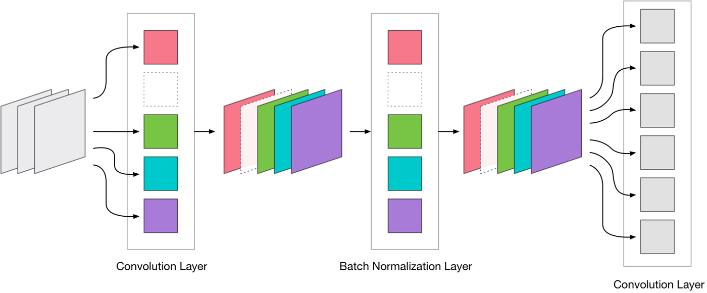
Instead of pruning away individual connectons we’ll remove complete convolution filters. This keeps our connections dense and the GPU happy.
Recall that a convolution layer produces an image with a certain number of output channels. Each of these output channels contains the result of a single convolution filter. Such a filter takes the weighted sum over all the input channels and writes this sum to a single output channel.
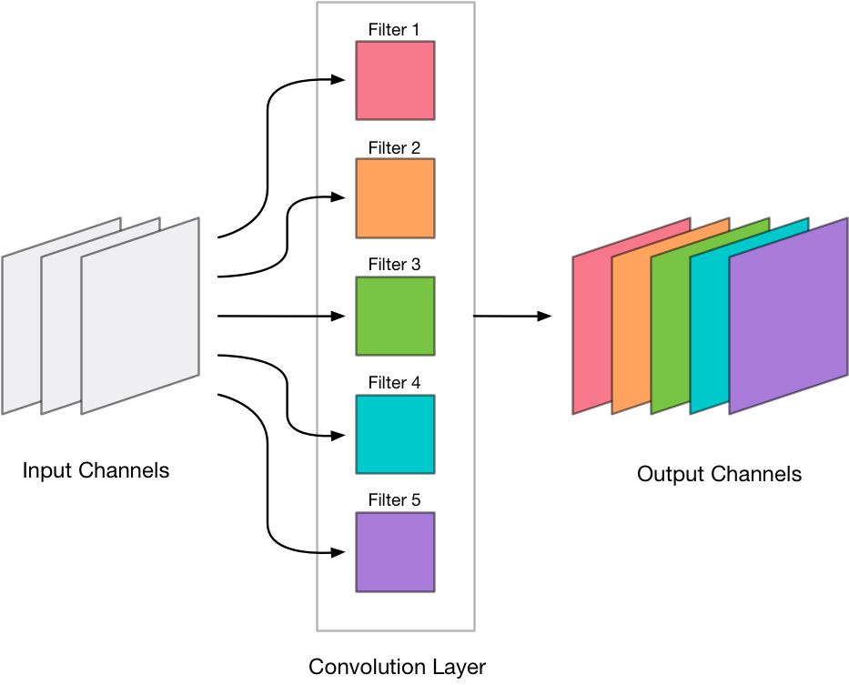
We’re going to find the convolution filters that are the least important and remove their output channels from the layer:
For example, layer conv_pw_12 in MobileNet has 1024 output channels. We’re going to throw away 256 of those channels so that the compressed version of conv_pw_12 only has 768 output channels.
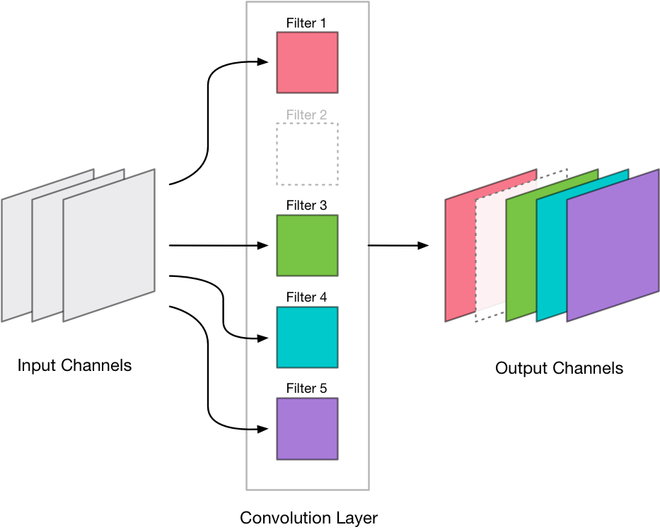
Note: To make Metal happy, we should always remove output channels four at a time. Because Metal is really a graphics API, it uses textures to describe the image data for the neural net, and each texture holds data for 4 consecutive channels. So if we were to remove just one output channel, Metal would still have to process that texture for the three other channels. Where Metal is concerned, compressing a layer only makes sense if we remove channels in multiples of four.
Now the question is: which filters / output channels do we remove? We only want to get rid of output channels that do not influence the final outcome too much.
There are different metrics you can use to estimate a filter’s relevance, but we’ll be using a very simple one: the L1-norm of the filter’s weights. If your math is a little rusty, it just means we take the absolute values of the filter’s weights and add them all up.
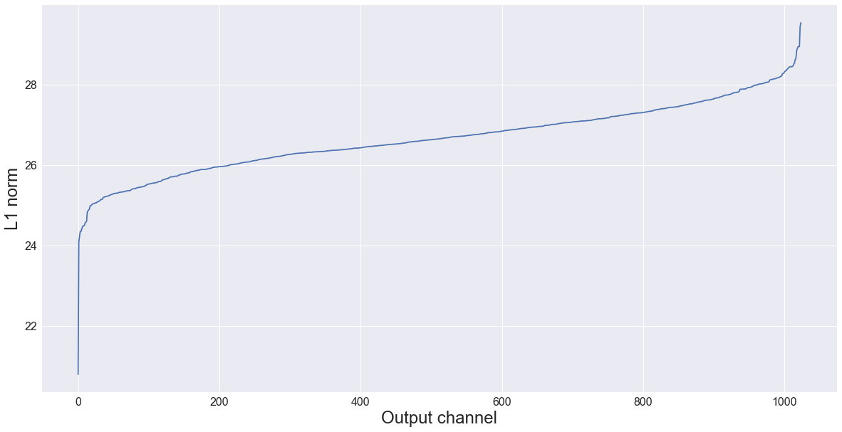
For example, these are the L1-norms of MobileNet’s very first convolution layer (32 filters), from low to high:
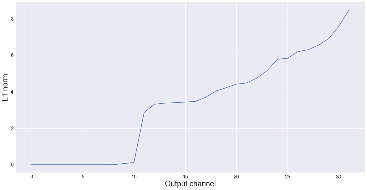
As you can see, there are about 10 filters in this first layer with an L1-norm that is very small — almost zero. We can probably get rid of these. But because the goal is to use this network with Metal, it doesn’t make sense to remove 10 filters. We have to remove either 8 or 12.
I first tried removing the 8 smallest filters. That worked so well — it gave no loss in accuracy at all — that I decided to drop the first 12 layers. As you’ll see shortly, that also worked just fine. That means we can actually remove 37.5% of the filters in the very first convolution layer in this network, without making the neural net worse!
Just for fun, here is a plot of the L1-norms of all the convolutional layers in MobileNet. You can see that many layers have filters that do not appear to contribute much to the network (low L1-norm).
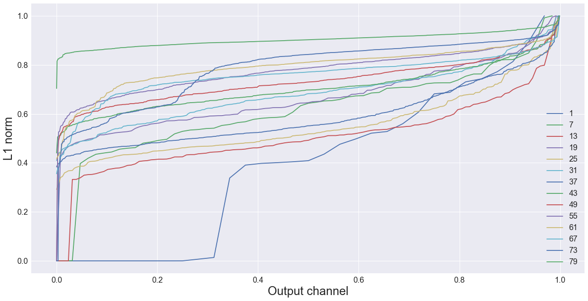
Note: Because not all layers have the same number of output channels, everything in this plot is normalized to be on the same scale. The horizontal axis represents the channels (sorted from low to high L1-norm), the vertical axis shows the actual L1-norms (also normalized).
You can read more about this approach in the paper Pruning Filters For Efficient Convnets by Li et al.
Removing filters from a layer means the number of output channels for that layer becomes smaller. Naturally, this has an effect on the next layer in the network too because that layer now receives fewer input channels.
As a result, we also have to remove the corresponding input channels from that layer. And when the convolution is followed by batch normalization, we also have to remove these channels from the batch norm parameters.
MobileNet actually has three kinds of convolutional layers:
- one regular 3×3 convolution (the very first layer)
- depth-wise convolutions
- 1×1 convolutions (also known as pointwise convolutions)
We can only remove filters from the 3×3 and 1×1 convolutions, but not from the depthwise ones. A depthwise convolution must always have the same number of output channels as it has input channels. There isn’t much to gain by compressing, and depthwise convolutions are pretty fast anyway (since they do way less work than a regular convolution). So we’ll primarily focus on the layers with 3×3 and 1×1 convolutions.
Retraining
Because removing filters from a layer makes the accuracy of the network worse — after all, you’re throwing away things that the neural net has learned, even if they may not be very important — you need to retrain the network a little, so that it can learn to compensate for the parts you just cut out.
Retraining just means you call model.fit() again. A little trial-and-error led me to a learning rate of 0.00001 — quite small, but anything larger made the training spin out of control. The reason the learning rate must be so small is that at this point the network is mostly trained already and we only want to make small changes to tweak the results.
The process then is:
- remove filters (i.e. output channels) from a layer, in multiples of 4
- retrain the network for a few epochs
- evaluate on the validation set to see if the network has regained its previous accuracy
- move to the next layer and repeat these steps
As you can tell, this process is quite labor-intensive, since we only compress one layer at a time and we need to retrain the network after every change. Figuring out how many filters to drop in each layer is not obvious either.
Using samples
MobileNet is trained on the dataset for the ILSVRC competition, also known as ImageNet. This is a huge dataset, consisting of over 1.2 million training images.
I recently built a modest deep learning rig (a Linux box with just one GTX 1080 Ti GPU). On this computer it takes 2 hours to train a single epoch. Even evaluating how well the network does on the 50,000-image validation set takes 3 minutes already.
Needless to say, this doesn’t allow for very rapid iterations. I didn’t want to twiddle my thumbs for 2 hours to see the effect of every tiny change. So instead, I decided to work on samples.
Instead of using the full training set, I picked 5 random images from each of the 1,000 categories (so that the sample is at least somewhat representative), which gives 5,000 training images in total. It now takes about 30 seconds to perform a single training epoch. That’s a lot more manageable than 2 hours!
For validation, I picked a random subset of 1,000 images from the full validation set. Evaluating the network on that subset only takes about 3 seconds.
It turned out that just using these samples worked really well in practice.
Compressing the first convolution layer
As you’ve seen, the first convolution layer has 10 filters with very small L1-norms. Since for Metal we need to remove filters in multiples of 4, I deleted the 12 filters with smallest L1-norms.
Initially, I didn’t actually remove any filters from the neural net at all, but just set the weights of their connections to 0. In theory that does the same thing. This made the top-1 accuracy drop from 69.4% to 68.7% — a bit less accurate but nothing that a little retraining can’t fix. Auspicious beginnings!
Next, I created a new model that had the same layers as the original, except here I physically removed the filters, so that the first convolution layer really only has 24 output channels instead of the original 36. But now the validation score was way worse: only 29.9% correct. Yikes, that is a big difference… What happened?
In theory, setting the weight of a connection to 0 should have the same effect as removing that connection. Well, it turns out that I messed up: I forgot to also set the weights for the corresponding input channels in the next layer to 0. But worse, since this next layer is a depthwise convolution, I also had to set the respective parameters for that layer’s batch normalization to 0.
Lesson learned: removing filters from one layer can have a big impact on the next several layers too. And the changes to those other layers also affect the validation score.
So was it a bad idea to remove 37.5% of the first conv layer’s filters? Well, upon inspection of the model, I found that all that was really “wrong” here were 12 bias values in the second batch norm layer — everything else becomes zero because it gets multiplied by something else that is zero, except those bias values.
And these 12 numbers made the difference between 68.7% accuracy and 29.9%. But… seriously?! On a neural net with 4 million parameters, these 12 numbers should not matter at all. With this insight, I felt confident that the network could recover from this 29.9% with some retraining.
I retrained the neural net on a training set sample (5,000 images) for 10 epochs (5 minutes of patience), and now the validation score was back up to 68.4%. That’s a little less than the original accuracy (69.4%) but close enough for now.
For this project, I’m happy if retraining on a sample brings the accuracy back to around 65%. Remember that the sample we’re retraining on is only 0.4% of the full training set size. I figure if such a small subset of training images can bring the accuracy almost back up to the original score, then adding in a few rounds of retraining on the full dataset at the end should get us all the way.
Note: It’s probably not a good idea to use the same training sample for too long. When you train for more than 10 or so epochs on the same sample, the network starts to seriously overfit on it. Whenever I retrained for more than 10 epochs, I usually refreshed the training sample.
Now, saving 37.5% of the weights from the first convolution layer sounds a like a lot but to be honest, it’s a very small layer. It has only 3 input channels and 32 output channels (now 24). Total savings: 3×3×3×12 = 324 parameters, a drop in the ocean. But hey, it’s a good start. Let’s keep going. 😅
The last pointwise conv layer
After compressing the first layer, I thought it would be a good idea to next try and compress the last convolution layer before the classification layer.
(In the Keras version of MobileNet the classification layer also happens to be a convolution layer, but we cannot remove any output channels from it. Since this network is trained on ImageNet, which has 1000 categories, the classification layer should also have 1000 output channels. If we were to remove any of these output channels, the model can no longer make predictions for those categories.)
The layer conv_pw_13 has 1024 output channels. I decided to remove 256 of those. Was there a well-though out argument behind this number? No, not really. But conv_pw_13 has 1,048,576 parameters. It is the largest layer in the network, so we can make big gains here.
The L1 norms for this layer look like this:
Hmm, judging from this plot maybe removing 256 channels is a bit much… but we’ll see. 😉
Again, we remove the output channels from the layer and the batch normalization layer that follows it, and then adjust the next layers so they also have fewer input channels.
Removing these 256 channels not only saves 1024×1×1×256 = 262,144 parameters on conv_pw_13, it also removes 256,000 parameters from the classification layer. Suddenly we’re cutting this sucker down!
After compressing the conv_pw_13 layer the validation score dropped to 60.7% (top-1) and 82.9% (top-5). That’s really not that bad, especially considering this is before any retraining.
After retraining for 10 epochs on a sample, the accuracy came up to 63.6%, and after another 10 epochs (on a new training sample) it was up to 65.0% (top-1) and 86.1% (top-5). Not bad for 10 minutes of training.
Getting a score like 0.65 makes me comfortable enough to move on to pruning additional layers. We’re not back up to the original score yet, but it shows that the network has successfully compensated for the pruned connections.
More layers & retraining for real
Next, I pruned conv_pw_10 (removed 32 out of 512 filters) and then conv_pw_12 (removed 256 out of 1024), using the same approach.
With every new layer I noticed that it became harder and harder for retraining to get the accuracy back up to previous standards. After conv_pw_10 it was 64.2%, after conv_pw_12 it was only 63.4%.
Each time I used a different training sample, just to make sure the results were still representative and the model wasn’t overfitting on the sample.
After pointwise layers 10 and 12, I did conv_pw_11. There really wasn’t a master plan behind the selection of which layers to compress when; I picked the layers somewhat arbitrarily.
On conv_pw_11 I pruned 96 out of 512 filters. For most of the other layers I had dropped 25% of the filters, roughly based on what the L1-norms were telling me, but mostly just because it’s a nice round number. Here, however, removing 128 filters caused the accuracy to drop off too much and retraining couldn’t get it over 60% again. Dropping “only” 96 filters gave better results, but even here the score was only 61.5% after retraining.
In the light of these disappointing validation scores, it’s definitely possible I have been too enthusiastic and removed too many filters so that now the neural net no longer has the capacity to learn ImageNet.
Up to this point all the retraining was done with “tiny” samples of 5,000 images, and so the pruned network has only been retrained on a fraction of the total training set. I decided it was time to subject the net to a few rounds of training on the full training set.
After 1 epoch, the accuracy was back up to 66.4 (top-1), 0.87 (top-5). I did not use data augmentation for this, only the original training images.
Since my GPU was already warmed up anyway, I decided to train for another epoch to see how much of a difference that would make. After this second epoch, the net scored 67.2 (top-1), 87.7 (top-5).
Just for kicks, I trained for a couple more epochs on the full training set, but with some data augmentation thrown in and with a smaller learning rate. Unfortunately, this did nothing to improve the results.
This is where I stopped the experiment, since I ran out of time. With another few rounds of training, I’m sure it would be possible to squeeze a few extra percentage points out of this network. And there are still nine pointwise convolution layers we haven’t touched yet — I’m sure we can drop a few filters from these layers that nobody would miss.
Conclusion
Original network size:   4,253,864 parameters
Compressed network size: 3,210,232 parameters
Compressed to:           75.5% of original size

Top-1 accuracy over 50000 images = 67.2%
Top-5 accuracy over 50000 images = 87.7%
The result is a little short of my goal: the network did become ~25% smaller but the accuracy is a little worse — but definitely not 25% worse!
The workflow could use some improvement, as I had to babysit the whole process. I also wasn’t very scientific about how I chose what filters to remove, or how I picked the order in which to compress the layers. But that’s OK… for this project, I just wanted to get an idea of what was possible.
Obviously, I did not arrive at an optimal pruning for this network. Using L1-norms may not be the best way to determine how important a filter is, and maybe it’s better to only remove a few filters at a time than to chop off 1/4th of the layer’s output channels in one go. But I am happy that using samples worked so well for retraining. Not having to wait hours for retraining means I could quickly run new experiments.
Is this sort of thing worth doing? I’d say so. Suppose you have a neural network that runs at 25 FPS on your iPhone, which means every frame takes 0.04 seconds to process. If the neural net is 25% smaller — and let’s assume this means it will also be 25% faster — then each frame will only take 0.03 seconds, which translates to over 30 FPS with some time to spare. This could be the difference between an app that runs choppy and an app that runs butter smooth.
Update 26 Feb 2018: I’ve been asked to share the source code, so here it is: Jupyter notebook on GitHub. Keep in mind this is still a work-in-progress. No guarantees. ;–)
First published on Saturday, 2 September 2017.
If you liked this post, say hi on Twitter @mhollemans or LinkedIn.
Find the source code on my GitHub.
 New e-book: Code Your Own Synth Plug-Ins With C++ and JUCE
Interested in how computers make sound? Learn the fundamentals of audio programming by building a fully-featured software synthesizer plug-in, with every step explained in detail. Not too much math, lots of in-depth information! Get the book at Leanpub.com