Google’s MobileNets on the iPhone

Sometime this April a very interesting paper titled MobileNets: Efficient Convolutional Neural Networks for Mobile Vision Applications appeared on arXiv.org.

The paper is written by a group of researchers at Google and introduces a neural network architecture called MobileNets.

The authors of the paper claim that this kind of neural network runs very efficiently on mobile devices and is nearly as accurate as much larger convolutional networks like our good friend VGGNet-16.

So of course I wanted to find out how fast it runs on the iPhone!

Depthwise separable convolutions

The big idea behind MobileNets: Use depthwise separable convolutions to build light-weight deep neural networks.

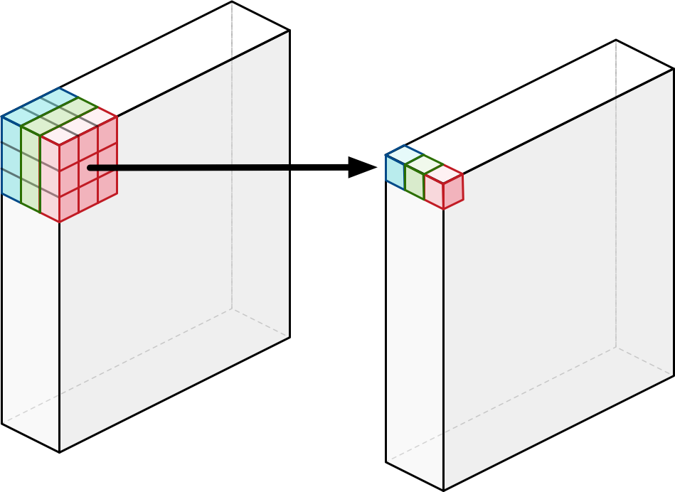
A regular convolutional layer applies a convolution kernel (or “filter”) to all of the channels of the input image. It slides this kernel across the image and at each step performs a weighted sum of the input pixels covered by the kernel across all input channels.

The important thing is that the convolution operation combines the values of all the input channels. If the image has 3 input channels, then running a single convolution kernel across this image results in an output image with only 1 channel per pixel.

So for each input pixel, no matter how many channels it has, the convolution writes a new output pixel with only a single channel. (In practice we run many convolution kernels across the input image. Each kernel gets its own channel in the output.)

The MobileNets architecture also uses this standard convolution, but just once as the very first layer. All other layers do “depthwise separable” convolution instead. This is actually a combination of two different convolution operations: a depthwise convolution and a pointwise convolution.

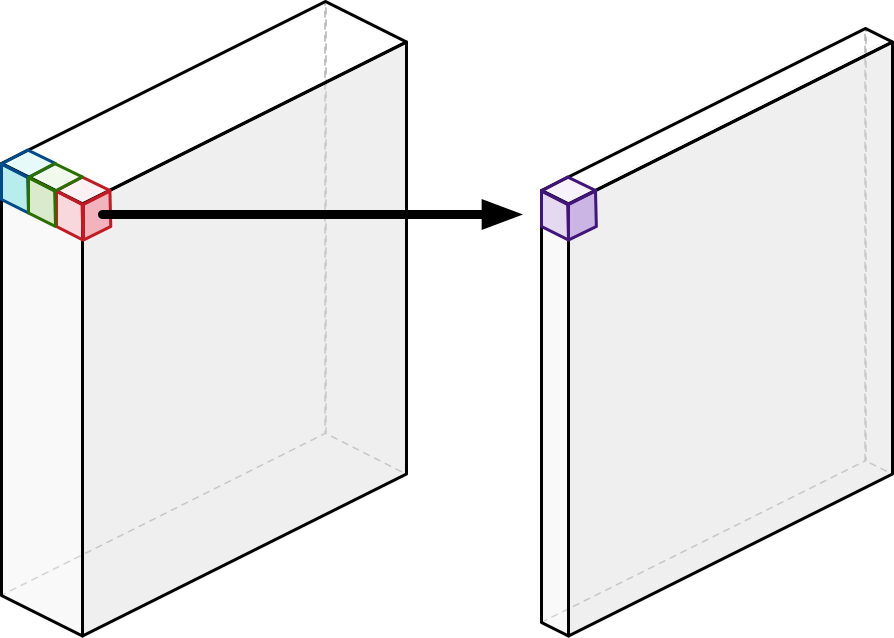
A depthwise convolution works like this:

Unlike a regular convolution it does not combine the input channels but it performs convolution on each channel separately. For an image with 3 channels, a depthwise convolution creates an output image that also has 3 channels. Each channel gets its own set of weights.

The purpose of the depthwise convolution is to filter the input channels. Think edge detection, color filtering, and so on.

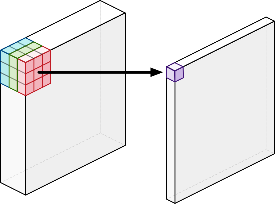
The depthwise convolution is followed by a pointwise convolution. This really is the same as a regular convolution but with a 1×1 kernel:

In other words, this simply adds up all the channels (as a weighted sum). As with a regular convolution, we usually stack together many of these pointwise kernels to create an output image with many channels.

The purpose of this pointwise convolution is to combine the output channels of the depthwise convolution to create new features.

When we put these two things together — a depthwise convolution followed by a pointwise convolution — the result is called a depthwise separable convolution. A regular convolution does both filtering and combining in a single go, but with a depthwise separable convolution these two operations are done as separate steps.

Why do this? The end results of both approaches are pretty similar — they both filter the data and make new features — but a regular convolution has to do much more computational work to get there and needs to learn more weights.

So even though it does (more or less) the same thing, the depthwise separable convolution is going to be much faster!

The paper shows the exact formula you can use to compute the speed difference but for 3×3 kernels this new approach is about 9 times as fast and still as effective. It’s no surprise therefore that MobileNets uses up to 13 of these depthwise separable convolutions in a row.

Using… MPSCNNDepthwiseConvolution?

Well, that’s going to be a bit of a problem. Metal does not support depthwise convolutions. 😢

I thought to be clever and use MPSCNNConvolution’s groups property for this. By setting groups to some value N, the convolution will apply separate filters to each group of N input channels. That sounds exactly what we want, but unfortunately the number of channels in each group must be a multiple of 4.

For our purposes we’d have to make groups equal to inputFeatureChannels but then the number of channels in each group is 1, which is not a multiple of 4. So this trick is not going to work.

That’s too bad, but no worries — we can always create our own layers.

Here’s an example of how to write a compute kernel for 3×3 depthwise convolution in the Metal Shading Language. It’s not optimized at all but it actually works quite well already:

kernel void depthwiseConv3x3_array(
  texture2d_array<half, access::sample> inTexture [[texture(0)]],
  texture2d_array<half, access::write> outTexture [[texture(1)]],
  constant KernelParams& params [[buffer(0)]],
  const device half4* weights [[buffer(1)]],
  const device half4* biasTerms [[buffer(2)]],
  ushort3 gid [[thread_position_in_grid]])
{
  // Make sure we don't write outside the output texture...
  if (gid.x >= outTexture.get_width() ||
      gid.y >= outTexture.get_height() ||
      gid.z >= outTexture.get_array_size()) return;

  constexpr sampler s(coord::pixel, filter::nearest, address::clamp_to_zero);

  // Each thread works on a single output pixel. Find which one that is.
  const ushort2 pos = gid.xy * stride;
  const ushort slices = outTexture.get_array_size();
  const ushort slice = gid.z;

  // Read the 3x3 block of pixels. Note that we read 4 channels at once.
  half4 in[9];
  in[0] = inTexture.sample(s, float2(pos.x - 1, pos.y - 1), slice);
  in[1] = inTexture.sample(s, float2(pos.x    , pos.y - 1), slice);
  in[2] = inTexture.sample(s, float2(pos.x + 1, pos.y - 1), slice);
  in[3] = inTexture.sample(s, float2(pos.x - 1, pos.y    ), slice);
  in[4] = inTexture.sample(s, float2(pos.x    , pos.y    ), slice);
  in[5] = inTexture.sample(s, float2(pos.x + 1, pos.y    ), slice);
  in[6] = inTexture.sample(s, float2(pos.x - 1, pos.y + 1), slice);
  in[7] = inTexture.sample(s, float2(pos.x    , pos.y + 1), slice);
  in[8] = inTexture.sample(s, float2(pos.x + 1, pos.y + 1), slice);

  // Take the weighted sum of the 3x3 pixels and our weights.
  // Again, note that we compute this for 4 channels at once.
  float4 out = float4(0.0f);
  for (ushort t = 0; t < 9; ++t) {
    out += float4(in[t]) * float4(weights[t*slices + slice]);
  }

  // Add a bias term and apply the ReLU.
  out += float4(biasTerms[slice]);
  out = applyNeuron(out, params.neuronA, params.neuronB);
  
  // Write the convolved pixel to the output image.
  outTexture.write(half4(out), gid.xy, gid.z);
}

I’m not going to explain in detail how this works but the above code snippet should give you some idea of what a depthwise convolution kernel does under the hood.

The MobileNets architecture

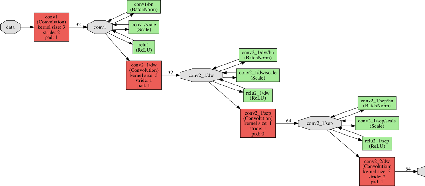
The full MobileNets network has 30 layers. The design of the network is quite straightforward:

1. convolutional layer with stride 2
2. depthwise layer
3. pointwise layer that doubles the number of channels
4. depthwise layer with stride 2
5. pointwise layer that doubles the number of channels
6. depthwise layer
7. pointwise layer
8. depthwise layer with stride 2
9. pointwise layer that doubles the number of channels

and so on…

After the very first layer (a regular convolution), the depthwise and pointwise layers take turns. Sometimes the depthwise layer has a stride of 2, to reduce the width and height of the data as it flows through the network. Sometimes the pointwise layer doubles the number of channels in the data. All the convolutional layers are followed by a ReLU activation function.

This goes on for a while until the original 224×224 image is shrunk down to 7×7 pixels but now has 1024 channels. After this there’s an average-pooling layer that works on the entire image so that we end up with a 1×1×1024 image, which is really just a vector of 1024 elements.

If we’re using MobileNets as a classifier, for example on ImageNet which has 1000 possible categories, then the final layer is a fully-connected layer with a softmax and 1000 outputs. If you wanted to use MobileNets on a different dataset, or as a feature extractor instead of classifier, you’d use some other final layer instead.

Even though MobileNets is designed to be pretty fast already, it’s possible to use a reduced version of this network architecture. There are three hyperparameters you can set that determine the size of the network:

• Width multiplier (the paper calls this “alpha”): this shrinks the number of channels. If the width multiplier is 1, the network starts off with 32 channels and ends up with 1024.

• Resolution multiplier (“rho” in the paper): this shrinks the dimensions of the input image. The default input size is 224×224 pixels.

• Shallow or deep. The full network has a group of 5 layers in the middle that you can leave out.

These settings can be used to make the network smaller — and therefore faster — but at the cost of prediction accuracy. (If you’re curious, the paper shows the effects of changing these hyperparameters on the accuracy.)

For the full network the total number of learned parameters is 4,221,032 (after folding the batch normalization layers). That’s certainly a lot less than VGGNet, which has over 130 million!

My implementation

You can find a version of MobileNets ready to go in the Forge repository on GitHub. Open Forge.xcworkspace in Xcode 8.3 or better and select the MobileNets target. You need to run this on an actual device with iOS 10.

The implementation of the neural net itself is in MobileNet.swift.

I had wanted to write this blog post back in April when the paper first came out, but at that point there was no pre-trained network available for MobileNets, and so the neural net could only compute nonsense. But recently I found this GitHub repo that has a version of MobileNets in Caffe — including a pre-trained network. Awesome!

Of course, Metal can’t read Caffe models directly, so I had to write a conversion script to convert the Caffe model to Metal. The conversion script also folds the batch normalization parameters into the convolution layers.

As is common with Caffe models, we need to do some preprocessing on the input image before we can give it to the neural net. That involves writing more Metal Shading Language code:

kernel void preprocess(
  texture2d<half, access::read> inTexture [[texture(0)]],
  texture2d<half, access::write> outTexture [[texture(1)]],
  uint2 gid [[thread_position_in_grid]])
{
  const auto inPixel = float4(inTexture.read(gid));
  const auto means = float4(123.68f, 116.78f, 103.94f, 0.0f);
  const auto inColor = (inPixel * 255.0f - means) * 0.017f;
  outTexture.write(half4(inColor.z, inColor.y, inColor.x, 0.0f), gid);
}

This compute kernel is invoked for every pixel in the input image. First, we read the input pixel (4 channels at a time). Then we multiply by 255.0f because Metal gives us the color in the range 0 – 1.

Next, we subtract the mean values for the red, green, and blue channels from the pixel. Then we scale by 0.017f. I’m not sure what purpose that serves, but that’s just how this network was trained. And finally, we flip the red and blue channels because Caffe models like to get their pixels in BGR order.

And that’s it, really… The main challenge was writing the compute kernel for the depthwise convolution, since Metal doesn’t have one. Other than that, the neural network is very straightforward. No funny stuff.

How fast is it?

The authors of the paper weren’t lying: MobileNets is fast!

Even with my unoptimized depthwise convolution, the full MobileNet architecture runs at about 0.05 seconds per image on the iPhone 6s. When let loose on a real-time video stream, the energy impact as measured by Xcode is medium to high.

So that’s 20 FPS at reasonable energy cost. Not bad for a deep neural net!

And on the new 10.5-inch iPad Pro it runs at 30 FPS with Xcode measuring only low energy impact. Very nice!

How does this compare to other neural networks? It’s about 3× as fast as Inception and 10× as fast as VGGNet-16, and it uses way less battery power than both. That’s largely due to the much smaller number of learned parameters (4 million versus 24 million for Inception-v3 and 138 million for VGGNet-16). Accessing memory is the biggest drain on battery power, so having many fewer parameters is a big plus.

Speed isn’t everything, of course. MobileNets is only useful if it’s also accurate. So how accurate is it?

The Caffe model I used was trained on the ImageNet data set. According to the paper, the top-1 validation accuracy for MobileNets on ImageNet is 70.6% versus 71.5% for VGGNet-16. The author of the Caffe model claims the version he trained “achieves slightly better accuracy rates than the original one reported in the paper”, a 70.81% top-1 accuracy (and 89.85% top-5) — so it comes quite close to VGGNet indeed.

That’s great because VGGNet-16 is often used as a feature extractor for other neural networks, so you can now simply replace that part of the network with this new MobileNets model and get an immediate 10× speed-up.

What about Core ML?

As you may have heard, the upcoming iOS 11 will have a brand new machine learning framework called Core ML. I was wondering how easy it would be to get MobileNets to run on Core ML. It turns out it was not very hard, once I figured out how to get the Core ML conversion tools up and running. 🤓

Here’s the GitHub repo with the code. It includes the conversion script as well, so you can see how I did the conversion (it’s only a few lines of code).

Unfortunately… the model only runs on the simulator but crashes on the device.

Long story short: Metal does not support depthwise convolutions. Well, I guess that’s no surprise (we already figured that out), but it also means MobileNets does not work with Core ML for the time being. If you’re interested in using MobileNets in your app, you’ll have to stick with MPS for a while.