
This blog post is a lightly edited chapter from my book Core ML Survival Guide.
If you’re interested in adding Core ML to your app, or you’re running into trouble getting your model to work, then check out the book. It’s filled with tips and tricks to help you make the most of the Core ML and Vision frameworks.
You can find the source code for this blog post in the book’s GitHub repo.
Enjoy!
* * *
In this blog post we’ll take a fairly complicated deep learning model and convert it to Core ML. This will use many of the techniques that were shown throughout the book, such as:
- converting a model
- cleaning up the model after conversion
- using
NeuralNetworkBuilderto create a new model - directly writing and modifying the spec
- building a pipeline to combine the different models into one
- using Vision to run the pipeline model in an iOS app
The model in question is SSD, which stands for Single Shot Multibox Detector — the M appears to have gone missing from the acronym. 😃
SSD is an object detector that is fast enough it can be used on real-time video.
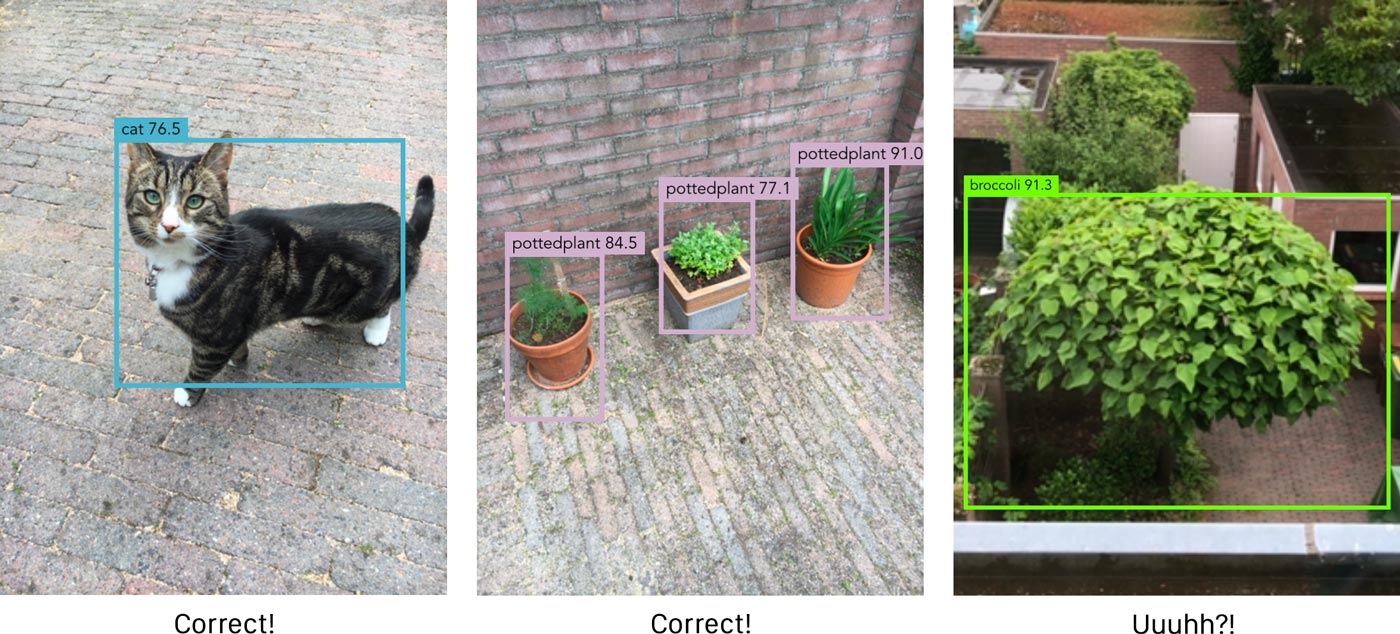
An object detector can find the locations of several different types of objects in the image. The detections are described by bounding boxes, and for each bounding box the model also predicts a class.
There are many variations of SSD. The one we’re going to use here employs MobileNet V2 as the backbone and has depthwise separable convolutions for the SSD layers, also known as SSDLite.
SSD vs. YOLO
SSD isn’t the only way to do real-time object detection. Another common model architecture is YOLO.
I wanted to mention YOLO because when you train an object detector with Turi Create, it produces a model with the TinyYOLO v2 architecture. The “tiny” YOLO model is smaller and therefore less accurate than the full one, but it’s also faster. Like SSD it was designed to run in real-time.
(Tiny)YOLO and SSD(Lite) work along the same lines. There are many architectural differences between them, but in the end both models make predictions on a fixed-size grid. Each cell in this grid is responsible for detecting objects in a particular location in the original input image.
It’s not super important that you understand the inner workings of these models. What matters is that they take an image as input and produce a tensor, or multi-array as Core ML calls it, of a certain size as output. This tensor contains the bounding box predictions in one form or another.
For an in-depth explanation of how these kinds of models work and how they are trained, see my blog post One-shot object detection.
The output tensor of TinyYOLO v2 is interpreted as a grid that has 13×13 cells. Turi Create’s version predicts 15 different bounding boxes per grid cell, or 13×13×15 = 2535 bounding boxes in total.
For SSDLite there are several different grids ranging in size from 19×19 to 1×1 cells. The number of bounding boxes per cell is 3 for the largest grid and 6 for the others, giving a total of 1917 boxes.
These models always predict the same number of bounding boxes, even if there is no object at a particular location in the image. To filter out the useless predictions, a post-processing step called non-maximum suppression (or NMS) is necessary.
In addition, the predictions aren’t of real bounding boxes but are relative to so-called anchor boxes. In order to turn the predictions into true rectangles, they must be decoded first. YOLO and SSD both use anchor boxes but have different ways of doing this.
Vision makes it easier
Until recently, the decoding and NMS post-processing steps had to be performed afterwards in Swift. The model would output an MLMultiArray containing the grid of predictions and you had to loop through the cells and perform these calculations yourself.
But as of iOS 12 and macOS 10.14, things have become a lot easier. The YOLO object detector from Turi Create is directly supported by the Vision framework.
You simply perform a Vision request on the image and the result is an array of VNRecognizedObjectObservation objects that contain the coordinates and class labels for the bounding boxes.
Vision automatically decodes the predictions for you and even performs NMS. How convenient is that!
The goal of this blog post is to create a version of MobileNetV2+SSDLite that works with Vision, just like Turi Create’s model does.
- First, we will convert the original model from TensorFlow to Core ML,
- then we’ll add operations that decode the predicted coordinates using the anchor boxes,
- and finally we’ll add NMS to the model as well.
Once all that is done, you can use SSD with Vision too — and get your hands on those precious VNRecognizedObjectObservation objects.
Converting from TensorFlow
We’ll be using the model ssdlite_mobilenet_v2_coco. You can download it here.
This model was trained using the TensorFlow Object Detection API and so we’ll need to use tfcoreml to convert it to Core ML.
If you don’t have tfcoreml installed yet, do so first:
pip3 install -U tfcoreml
The conversion process will give us a version of SSD that will work with Core ML but you won’t be able to use it with the new Vision API just yet.
Note: The following instructions were tested with coremltools 2.0, tfcoreml 0.3.0, and TensorFlow 1.7.0. If you’re using different versions of any of these packages, you may also get different results. Especially tfcoreml is being updated and improved regularly, so some of the issues we’ll encounter here may have been fixed in later versions.
The ssdlite_mobilenet_v2_coco download contains the trained SSD model in a few different formats: a frozen graph, a checkpoint, and a SavedModel. tfcoreml needs to use a frozen graph but the downloaded one gives errors — it contains “cycles” or loops, which are a no-go for tfcoreml. We’ll use the SavedModel and convert it to a frozen graph without cycles.
First, load the SavedModel into a new TensorFlow graph object:
import tensorflow as tf
from tensorflow.python.tools import strip_unused_lib
from tensorflow.python.framework import dtypes
from tensorflow.python.platform import gfile

def load_saved_model(path):
    the_graph = tf.Graph()
    with tf.Session(graph=the_graph) as sess:
        tf.saved_model.loader.load(sess,
                [tf.saved_model.tag_constants.SERVING], path)
    return the_graph

saved_model_path = "ssdlite_mobilenet_v2_coco_2018_05_09/saved_model"
the_graph = load_saved_model(saved_model_path)
Next, we’ll use a helper function to strip away unused subgraphs and save the result as another frozen model:
frozen_model_file = "frozen_model.pb"
input_node = "Preprocessor/sub"
bbox_output_node = "concat"
class_output_node = "Postprocessor/convert_scores"

def optimize_graph(graph):
    gdef = strip_unused_lib.strip_unused(
            input_graph_def = graph.as_graph_def(),
            input_node_names = [input_node],
            output_node_names = [bbox_output_node, class_output_node],
            placeholder_type_enum = dtypes.float32.as_datatype_enum)

    with gfile.GFile(frozen_model_file, "wb") as f:
        f.write(gdef.SerializeToString())

optimize_graph(the_graph)
The strip_unused() function will only keep the portion of the graph in between the specified input and output nodes, and removes everything else. What’s left is the only piece of the original graph that Core ML can actually handle — the rest is full of unsupported operations.
The part of the TensorFlow graph that we keep has one input for the image and two outputs: one for the bounding box coordinate predictions and one for the classes. While YOLO combines the coordinate and class predictions into a single tensor, SSD makes these predictions on two separate branches. That’s why we also have to supply the names of two output nodes.
I looked up these node names in the saved_model.pb file using Netron.
TensorFlow models can be quite complicated, so it usually takes a bit of searching to find the nodes you need. Another trick is to simply print out a list of all the operations in the graph and look for ones that seem reasonably named, then run the graph up to that point and see what sort of results you get.
Note: By the way, I didn’t come up with this code myself — it’s taken from this tfcoreml example notebook. Interestingly, they use a different output node. SSD does multi-label classification on the class predictions, which applies a sigmoid activation to the class scores. The node that they use, "concat_1", happens before the sigmoid, while "Postprocessor/convert_scores" is after the sigmoid. By including this node it saves us from having to apply the sigmoid ourselves.
Now we’ve got something that tfcoreml will be happy with. To convert the frozen TensorFlow graph to Core ML, do the following:
import tfcoreml

coreml_model_path = "MobileNetV2_SSDLite.mlmodel"

input_width = 300
input_height = 300

input_tensor = input_node + ":0"
bbox_output_tensor = bbox_output_node + ":0"
class_output_tensor = class_output_node + ":0"

ssd_model = tfcoreml.convert(
    tf_model_path=frozen_model_file,
    mlmodel_path=coreml_model_path,
    input_name_shape_dict={ input_tensor: [1, input_height, input_width, 3] },
    image_input_names=input_tensor,
    output_feature_names=[bbox_output_tensor, class_output_tensor],
    is_bgr=False,
    red_bias=-1.0,
    green_bias=-1.0,
    blue_bias=-1.0,
    image_scale=2./255)
This is fairly straightforward usage of tfcoreml. We specify the same inputs and output names again but this time they need to have the :0 appended.
The expected size of the input image is 300×300 pixels. Fun fact: YOLO uses larger images of 416×416 pixels.
The image preprocessing options are typical for TensorFlow image models: first divide by 127.5 to put the pixels in the range [0, 2], then subtract -1 to put them in the range [-1, 1].
Often TensorFlow models already do their own normalization and this one is no exception. However, when we stripped away the parts of the model we couldn’t use, such as anything before the input node "Preprocessor/sub:0", we also got rid of the original model’s built-in preprocessing operations.
After a few brief moments, if all goes well, tfcoreml completes the conversion and saves the mlmodel to a file. We now have a Core ML model that takes a 300×300 image as input and produces two outputs: a multi-array with the coordinates for 1917 bounding boxes and another multi-array with the class predictions for the same 1917 bounding boxes.
Note: At this point, the predicted coordinates aren’t “real” coordinates yet — they still have to be decoded using the anchor boxes. Also remember the model always predicts 1917 bounding boxes for any image. Most of these bounding boxes will not have detected an actual object. In that case, the class “unknown” has the highest score. We’ll later use non-maximum suppression to filter out these predictions.
Cleaning it up
In theory we could start using the converted model already, but I always like to clean up the converted model first.
Due to how the input and output tensors were named in the original model, the Core ML model’s input is named "Preprocessor__sub__0" while the two outputs are "Postprocessor__convert_scores__0" and "concat__0". Those are pretty meaningless — and ugly! — names.
Let’s rename the input to "image" and the two outputs to "scores" and "boxes", respectively. This requires using the model’s spec object:
spec = ssd_model.get_spec()

spec.description.input[0].name = "image"
spec.description.input[0].shortDescription = "Input image"
spec.description.output[0].name = "scores"
spec.description.output[0].shortDescription = "Predicted class scores for each bounding box"
spec.description.output[1].name = "boxes"
spec.description.output[1].shortDescription = "Predicted coordinates for each bounding box"
It’s not enough to change these names in the spec.description. Any layers that are connected to the old input or output names must now use the new names too. Likewise for the object that handles the image preprocessing.
input_mlmodel = input_tensor.replace(":", "__").replace("/", "__")
class_output_mlmodel = class_output_tensor.replace(":", "__").replace("/", "__")
bbox_output_mlmodel = bbox_output_tensor.replace(":", "__").replace("/", "__")

for i in range(len(spec.neuralNetwork.layers)):
    if spec.neuralNetwork.layers[i].input[0] == input_mlmodel:
        spec.neuralNetwork.layers[i].input[0] = "image"
    if spec.neuralNetwork.layers[i].output[0] == class_output_mlmodel:
        spec.neuralNetwork.layers[i].output[0] = "scores"
    if spec.neuralNetwork.layers[i].output[0] == bbox_output_mlmodel:
        spec.neuralNetwork.layers[i].output[0] = "boxes"

spec.neuralNetwork.preprocessing[0].featureName = "image"
If we look at the outputs using print(spec.description), the "scores" output correctly shows up as a multi-array but its shape is not filled in:
  type {
    multiArrayType {
      dataType: DOUBLE
    }
  }
We know for a fact that this always outputs an array of shape (91, 1917) because there are 91 classes and 1917 bounding boxes. Why 91 classes? This model was trained on the COCO dataset and so it can detect 90 possible types of objects, plus one class for “no object detected”.
Let’s remedy that and fill in the output shape:
num_classes = 90
num_anchors = 1917
spec.description.output[0].type.multiArrayType.shape.append(num_classes + 1)
spec.description.output[0].type.multiArrayType.shape.append(num_anchors)
Note that we define num_classes to be 90, not 91, because we want to ignore the bounding boxes that did not detect anything. In fact, later on we’ll remove any such detections for this “unknown” class from the model completely.
The "boxes" output’s shape has something wrong with it too:
  multiArrayType {
    shape: 4
    shape: 1917
    shape: 1
    dataType: DOUBLE
  }
The first two dimensions are correct, but there is no reason to have that third dimension of size 1, so we might as well get rid of it:
del spec.description.output[1].type.multiArrayType.shape[-1]
Note: The model will work fine even when the output shapes aren’t filled in completely or even incorrectly. But the shape also serves as documentation for the user of the model, and so I like to make sure it is right.
Finally, let’s convert the weights to 16-bit floats:
import coremltools
spec = coremltools.utils.convert_neural_network_spec_weights_to_fp16(spec)
And save the model again. We could just save the spec, but it’s easier to create a new MLModel object — and we’ll need this later to build the pipeline anyway.
ssd_model = coremltools.models.MLModel(spec)
ssd_model.save(coreml_model_path)
Now if you open MobileNetV2_SSDLite.mlmodel in Xcode, it shows the following:

The input is a 300×300-pixel image and there are two multi-array outputs.
The scores output is pretty straightforward to interpret: for every one of the 1917 bounding boxes there is a 91-element vector containing a multi-label classification.
However, in order to use this model in an app, you still need some way to make sense out of the predicted bounding box “coordinates” from the boxes output…
Decoding the bounding box predictions
As I mentioned before, the values coming out of the boxes output are not real coordinates yet. Instead, these numbers describe how to modify the anchor boxes.
An anchor box is nothing more than a pre-defined rectangle that is located somewhere in the original image. It is described by four numbers: x, y, width, and height. There are 1917 unique anchor boxes, one for each prediction from boxes.
The purpose of the anchor boxes is to give the model some idea of what sizes of objects to look for. The anchor boxes represent the most common (rectangular) shapes among the objects in the dataset. They act as hints for the model during the training process — without these anchor boxes, it’s much harder for the model to learn its objective.
The four numbers that SSD predicts for each bounding box describe how the position and size of the corresponding anchor box should be modified in order to fit the detected object. For example, the predicted numbers may say, “move my anchor box 20 pixels to the left, and make it 5% wider but also 3% less tall.”
The model is trained to make its prediction using the anchor box that best fits the detected object, and then tweak the box a little so that it fits perfectly.
The anchor boxes are chosen prior to training and are always fixed. In other words, they are a hyperparameter. The original YOLO ran a clustering algorithm on the training set to determine the most common object shapes, but SSD and also Turi Create use a simple mathematical formula for selecting the positions and sizes of the anchor boxes.
To be able to decode the coordinate predictions, we first need to know what the anchor boxes are. It’s possible to dig up the mathematical formula for computing the anchor box positions and sizes — but as this formula is part of the original TensorFlow model, we can also simply ask the graph:
import numpy as np

def get_anchors(graph, tensor_name):
    image_tensor = graph.get_tensor_by_name("image_tensor:0")
    box_corners_tensor = graph.get_tensor_by_name(tensor_name)
    box_corners = sess.run(box_corners_tensor, feed_dict={
        image_tensor: np.zeros((1, input_height, input_width, 3))})

    ymin, xmin, ymax, xmax = np.transpose(box_corners)
    width = xmax - xmin
    height = ymax - ymin
    ycenter = ymin + height / 2.
    xcenter = xmin + width / 2.
    return np.stack([ycenter, xcenter, height, width])

anchors_tensor = "Concatenate/concat:0"
with the_graph.as_default():
    with tf.Session(graph=the_graph) as sess:
        anchors = get_anchors(the_graph, anchors_tensor)
Note: This is one of the reasons why tfcoreml cannot convert the original frozen model: because of the operations that generate the anchor boxes. We first had to remove those operations from the graph.
To get the appropriate anchor boxes for our desired input image size, we must run the graph on such an image. Here we’re simply using a fake image that is all zeros. For the anchor boxes it doesn’t matter what is actually in the image, only how large it is (300×300 pixels in our case).
The TensorFlow graph computes each anchor box as the rectangle (ymin, xmin, ymax, xmax). We convert these min/max values to a center coordinate plus width and height. By the way, the anchor box coordinates are normalized, i.e. between 0 and 1, so that they are independent of the original image size.
After you run this code, anchors is a NumPy array of shape (4, 1917). There is exactly one anchor box for each bounding box prediction, described by the four numbers (y, x, height, width).
Yes, that’s a little weird — you probably expected it to be (x, y, width, height) — but this is a TensorFlow convention.
Before the introduction of the new Vision VNRecognizedObjectObservation API, you would’ve had to save the anchors array to a file and load it into your app. Your Swift code would then need to do the following to decode the predictions into real coordinates:
for b in 0..<numAnchors {
  // Read the anchor coordinates:
  let ay = anchors[b               ]
  let ax = anchors[b + numAnchors  ]
  let ah = anchors[b + numAnchors*2]
  let aw = anchors[b + numAnchors*3]

  // Read the predicted coordinates:
  let ty = boxes[b               ]
  let tx = boxes[b + numAnchors  ]
  let th = boxes[b + numAnchors*2]
  let tw = boxes[b + numAnchors*3]

  // The decoding formula:
  let x = (tx / 10) * aw + ax
  let y = (ty / 10) * ah + ay
  let w = exp(tw / 5) * aw
  let h = exp(th / 5) * ah

  // The final bounding box is given by (x, y, w, h)
}
Here, numAnchors is 1917. This code snippet loops through each predicted box and applies a simple formula involving exp() and some arithmetic to get the decoded coordinates.
You could optimize this logic using the vectorized functions from the Accelerate framework, or even implement it as a custom layer in the Core ML model. This is a massively parallel computation — the exact same formula is applied to each of the 1917 predictions — and so it’s well suited to running on the GPU.
But I want to use the shiny new Vision API! 😍 And so we’re going to take another approach and add this logic to the mlmodel itself using built-in Core ML operations.
Note: The above decoding formula is unique to SSD. For YOLO you also need to decode the predictions but the calculations are slightly different.
Decoding inside the Core ML model
Adding the decoding logic to the mlmodel involves taking the above formula and implementing it using various Core ML layer types.
We could directly add these layers to the SSD model that we just converted, but instead let’s create a completely new model from scratch. Later, we’ll connect these models together using a pipeline.
The easiest way to build this decoder model is to use NeuralNetworkBuilder:
from coremltools.models import datatypes
from coremltools.models import neural_network

input_features = [
    ("scores", datatypes.Array(num_classes + 1, num_anchors, 1)),
    ("boxes", datatypes.Array(4, num_anchors, 1))
]

output_features = [
    ("raw_confidence", datatypes.Array(num_anchors, num_classes)),
    ("raw_coordinates", datatypes.Array(num_anchors, 4))
]

builder = neural_network.NeuralNetworkBuilder(input_features, output_features)
The inputs to the decoder model are exactly the same as the outputs from the SSD model. Well, almost. The boxes output from SSD has shape (4, num_anchors) but here we say the shape is (4, num_anchors, 1). Similarly for the scores output.
In Core ML, if the input to a neural network model is a multi-array it must have either one or three dimensions. Since our arrays only have two dimensions, we need to add an unused dimension of size 1 at the front or back. ¯\_(ツ)_/¯
The outputs of the decoder model are very similar to its inputs, except that the order of the dimensions has been flipped around. There are only two dimensions now, and the number of bounding boxes is in the first dimension. The next step in the pipeline, non-maximum suppression, demands it that way.
Note: Even though the input multi-arrays are not allowed to have two dimensions, this is fine for the outputs. The NonMaximumSuppression model is not a neural network, so it doesn’t have that restriction.
Also notice that we use num_classes for the decoder output, not num_classes + 1. We’re not interested in bounding boxes that do not belong to any object and so the decoder will ignore predictions for the “unknown” class.
SSD does multi-label classification, which means that the same bounding box can have more than one class. Any class whose predicted probability is over a certain “confidence threshold” counts as a valid prediction. For the vast majority of the 1917 predicted bounding boxes, the “unknown” class will have a high score and all the other classes will have scores below the threshold.
Note: With YOLO / Turi Create this is a bit different. YOLO’s classification is multi-class (softmax), not multi-label (sigmoid). It also predicts a separate confidence score for the bounding box itself, which indicates whether YOLO thinks this bounding box contains an object or not. In SSD this is represented by the score for the “unknown” class. The confidence score for the bounding box is multiplied with the probability for the highest scoring class. If that combined confidence score is over a certain threshold, the bounding box is kept.
All right, let’s build this decoder model. First let’s look at the scores input. The decoder needs to do two things with the scores:
- swap around the dimensions, and
- strip off the predictions for the “unknown” class.
To swap the dimensions we use a permute operation:
builder.add_permute(name="permute_scores",
                    dim=(0, 3, 2, 1),
                    input_name="scores",
                    output_name="permute_scores_output")
Even though our input is a tensor with three dimensions, (91, 1917, 1), the permute layer treats it as having four dimensions. The first dimension is used for sequences and we’ll leave it alone.
After permuting, the shape of the data is now (1, 1, 1917, 91). Each bounding box prediction gets a 91-element vector with the class scores, the first of which is the prediction for class “unknown”. To strip this off we use a slice operation that works on the “width” axis (the last one). We only want to keep the elements 1 through 90, so we set start_index=1 and end_index=91 (the end index is exclusive):
builder.add_slice(name="slice_scores",
                  input_name="permute_scores_output",
                  output_name="raw_confidence",
                  axis="width",
                  start_index=1,
                  end_index=num_classes + 1)
Now the data has shape (1, 1, 1917, 90). That tensor can go straight into the decoder model’s first output, "raw_confidence". Note that we declared this output to have shape (1917, 90). The first two dimensions are automatically dropped by Core ML because they are of size 1.
Next up is the second input, boxes, that has the bounding box “coordinates”. As I mentioned in the previous section, the formula for decoding a single bounding box is as follows,
x = (tx / 10) * aw + ax
y = (ty / 10) * ah + ay
w = exp(tw / 5) * aw
h = exp(th / 5) * ah
where tx, ty, tw, th are the predictions from SSD and ax, ay, aw, ah are the anchor box coordinates. This happened in a for loop. Seems simple enough, except in Core ML we can’t have loops, so we’ll have to work on the entire tensor at once.
The shape of the boxes tensor is (4, 1917, 1). Recall that we had to add that extra dimension in order to make this input three dimensional. Since adding a dimension of size 1 doesn’t change the data, we could have added it to the front, but we put it in the back for a good reason: we want the coordinates to be in what Core ML calls the “channel” dimension. This is important for later on when we need to use a concatenation layer.
It doesn’t really matter much where the 1917 goes, it can go either in the “height” dimension or the “width” dimension. I put these terms inside quotes because it is only by convention that they’re named that way and we’re not using them for that purpose right now.
Let’s start with the x and y coordinates. According to the decoding formula, we must divide these by 10. But we can’t simply apply the division operation on the entire boxes array because that would also change the width and height (these need to be divided by 5 instead). So first, we grab only the x and y coordinates by slicing up the array:
builder.add_slice(name="slice_yx",
                  input_name="boxes",
                  output_name="slice_yx_output",
                  axis="channel",
                  start_index=0,
                  end_index=2)
Since the coordinates are in the “channels” dimension, that’s what we put for axis. Here we’re slicing off the first two channels.
Notice that I called this layer "slice_yx" with y coming before x. That’s because SSD’s prediction of the 4 coordinates is in the order (y, x, height, width). The anchor box coordinates are also stored in this order.
It doesn’t really matter one way or the other what the chosen order is, as long as we’re careful to use the correct one. The non-maximum suppression requires that the decoder model outputs bounding boxes for which the coordinates are given as (x, y, width, height), so at some point we’ll have to flip y and x, height and width.
Now that we’ve isolated the y/x coordinates, we can divide them by the scalar constant 10. In Core ML you can do this by using a multiply layer. Normally this performs element-wise multiplication between the tensors from two inputs, but if you only supply one input it multiplies every element in that tensor with a constant value.
builder.add_elementwise(name="scale_yx",
                        input_names="slice_yx_output",
                        output_name="scale_yx_output",
                        mode="MULTIPLY",
                        alpha=0.1)
Next up comes an interesting challenge: We must now multiply the “x” result with aw, the width of the anchor box, and the “y” result with ah, the height of the anchor box. That means we need to put these anchor box coordinates into the Core ML model somehow. The operator for this is load constant.
Earlier we retrieved the anchor boxes from the TensorFlow graph. The anchors variable contains a NumPy array of shape (4, 1917). We need to split this up into two arrays of shape (2, 1917, 1). One array contains the y, x coordinates of the anchor boxes, the other their heights and widths.
We can do this with NumPy slicing:
anchors_yx = np.expand_dims(anchors[:2, :], axis=-1)
anchors_hw = np.expand_dims(anchors[2:, :], axis=-1)
Notice that these new arrays have an empty dimension of 1 at the end. That’s what expand_dims() is for. We’re doing this because the tensors also have the shape (2, 1917, 1).
Let’s add both of these anchors arrays into the Core ML model:
builder.add_load_constant(name="anchors_yx",
                          output_name="anchors_yx",
                          constant_value=anchors_yx,
                          shape=[2, num_anchors, 1])

builder.add_load_constant(name="anchors_hw",
                          output_name="anchors_hw",
                          constant_value=anchors_hw,
                          shape=[2, num_anchors, 1])
Now we’ll perform an element-wise multiplication between "anchors_hw" and the output from "scale_yx":
builder.add_elementwise(name="yw_times_hw",
                        input_names=["scale_yx_output", "anchors_hw"],
                        output_name="yw_times_hw_output",
                        mode="MULTIPLY")
And then we’ll do an element-wise addition with the values from "anchors_yx":
builder.add_elementwise(name="decoded_yx",
                        input_names=["yw_times_hw_output", "anchors_yx"],
                        output_name="decoded_yx_output",
                        mode="ADD")
That completes the formula for the y and x coordinates. We’ve divided by 10 — or actually multiplied by 1⁄10 — also have multiplied by the anchor height/width, and added the anchor center position.
We still have to calculate the true height and width of the predicted bounding box. This happens in a very similar manner. First, we slice off the height and width from the original boxes tensor (the last two channels), then divide these predictions by 5 using a multiply layer with alpha=0.2:
builder.add_slice(name="slice_hw",
                  input_name="boxes",
                  output_name="slice_hw_output",
                  axis="channel",
                  start_index=2,
                  end_index=4)

builder.add_elementwise(name="scale_hw",
                        input_names="slice_hw_output",
                        output_name="scale_hw_output",
                        mode="MULTIPLY",
                        alpha=0.2)
Next, we use a unary function layer to exponentiate these values:
builder.add_unary(name="exp_hw",
                  input_name="scale_hw_output",
                  output_name="exp_hw_output",
                  mode="exp")
And finally, we multiply by the anchor height and width:
builder.add_elementwise(name="decoded_hw",
                        input_names=["exp_hw_output", "anchors_hw"],
                        output_name="decoded_hw_output",
                        mode="MULTIPLY")
Great, that was all the math we needed for decoding the predictions using the anchor boxes. But we’re not done yet!
We have two tensors now, both of size (2, 1917, 1). These need to be combined into one big tensor of size (1917, 4). That will involve concatenation and a permutation of some kind.
But there is a small wrinkle: if we were to simply use a concat layer to put the two tensors together, then the order of the coordinates is (y, x, height, width) — but we need them as (x, y, width, height).
So instead, we’ll slice them up into four separate tensors of size (1, 1917, 1) and then concatenate these in the right order.
builder.add_slice(name="slice_y",
                  input_name="decoded_yx_output",
                  output_name="slice_y_output",
                  axis="channel",
                  start_index=0,
                  end_index=1)

builder.add_slice(name="slice_x",
                  input_name="decoded_yx_output",
                  output_name="slice_x_output",
                  axis="channel",
                  start_index=1,
                  end_index=2)

builder.add_slice(name="slice_h",
                  input_name="decoded_hw_output",
                  output_name="slice_h_output",
                  axis="channel",
                  start_index=0,
                  end_index=1)

builder.add_slice(name="slice_w",
                  input_name="decoded_hw_output",
                  output_name="slice_w_output",
                  axis="channel",
                  start_index=1,
                  end_index=2)

builder.add_elementwise(name="concat",
                        input_names=["slice_x_output", "slice_y_output",
                                     "slice_w_output", "slice_h_output"],
                        output_name="concat_output",
                        mode="CONCAT")
Now we can permute this from (4, 1917, 1) to (1, 1917, 4) and write the results to the second output of the decoder model, "raw_coordinates":
builder.add_permute(name="permute_output",
                    dim=(0, 3, 2, 1),
                    input_name="concat_output",
                    output_name="raw_coordinates")
The final predicted bounding box coordinates are already normalized, meaning that they are between 0 and 1 (although they can be slightly smaller or larger too). That’s good, because the next stage, non-maximum suppression, expects them that way.
For other types of models that don’t use normalized coordinates, you might need to do some extra arithmetic to scale the bounding box coordinates down. Turi’s YOLO model, for example, has a scale layer at the end that divides the coordinates by 13 to normalize them.
Now that we’re done building the decoder, let’s turn it into an actual MLModel and save it:
decoder_model = coremltools.models.MLModel(builder.spec)
decoder_model.save("Decoder.mlmodel")
We don’t really need to save this model, as we’ll put it into a pipeline shortly, but sometimes coremltools will crash the Python interpreter and it’s nice to not have to repeat all the work we just did.
Just for fun, this is what the model looks like in Netron:
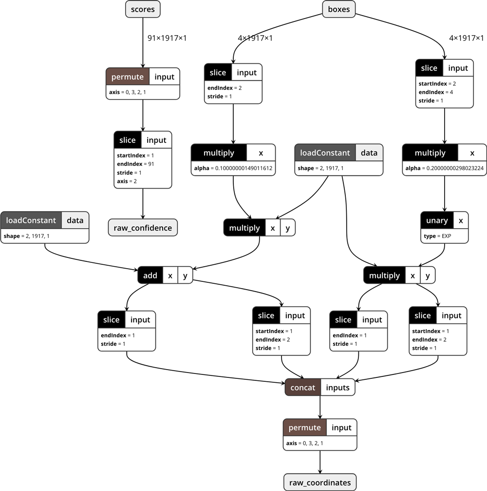
Tip: It’s useful to occasionally save the model and inspect it with Netron while you’re developing it, to make sure all the layers are connected properly etc. In that case it’s best to save the model using coremltools.utils.save_spec(builder.spec, "Decoder.mlmodel"), as creating the MLModel object is one of the things that tends to crash Python if there is a problem with your model definition.
Non-maximum suppression
The third and final model we’ll build is the one for non-maximum suppression. In Core ML this is not a neural network layer but a separate model type. There is no convenient API for building this kind of model, so we’ll have to write some protobuf code by hand:
nms_spec = coremltools.proto.Model_pb2.Model()
nms_spec.specificationVersion = 3
The specification version needs to be 3 because that’s the earliest version of the mlmodel format that supports non-maximum suppression.
First, we need to define the inputs and outputs for this model. Because the inputs must be the same as the decoder model’s outputs, we can simply copy over their definitions:
for i in range(2):
    decoder_output = decoder_model._spec.description.output[i].SerializeToString()

    nms_spec.description.input.add()
    nms_spec.description.input[i].ParseFromString(decoder_output)

    nms_spec.description.output.add()
    nms_spec.description.output[i].ParseFromString(decoder_output)

nms_spec.description.output[0].name = "confidence"
nms_spec.description.output[1].name = "coordinates"
Because non-maximum suppression may return a different number of bounding boxes for every input image, we should make the output shapes flexible.
The confidence and coordinates outputs may have anywhere from 0 to 1917 bounding boxes, but right now their sizes are fixed to always return the maximum of 1917 predictions.
Normally you’d use the helper functions from the flexible_shape_utils module but these are really meant for changing the inputs and outputs of neural network models. But this isn’t going to be a neural network, so we’ll have to modify the spec ourselves:
output_sizes = [num_classes, 4]
for i in range(2):
    ma_type = nms_spec.description.output[i].type.multiArrayType
    ma_type.shapeRange.sizeRanges.add()
    ma_type.shapeRange.sizeRanges[0].lowerBound = 0
    ma_type.shapeRange.sizeRanges[0].upperBound = -1
    ma_type.shapeRange.sizeRanges.add()
    ma_type.shapeRange.sizeRanges[1].lowerBound = output_sizes[i]
    ma_type.shapeRange.sizeRanges[1].upperBound = output_sizes[i]
    del ma_type.shape[:]
The first dimension from each output represents the number of bounding boxes that will be returned.
We set the lower bound for this dimension to 0, so the minimum predicted amount is no bounding boxes. This happens when none of the boxes has a predicted class score that is over the confidence threshold.
The upper bound is -1, meaning there is no limit to the maximum number of predictions — although you’ll never get more than 1917 results, and in practice it’s usually less than 10 or so.
The second dimension of the output tensor is not flexible at all because the lower bound and upper bound are equal here. For the confidence output it is always num_classes (90), for the coordinates output it’s always 4.
We also remove the old fixed-size shape information from the outputs using del ma_type.shape[:] because that conflicts with the flexible size ranges.
Tip: In order to figure out how to do this sort of thing, I spent some time reading through the Turi Create source code, notably the method export_coreml(). Recommended practice for anyone who wants to learn how to build advanced Core ML models!
Now let’s turn this into a model of type NonMaximumSuppression. You can find the full definition of this model type in NonMaximumSuppression.proto. We begin by filling out the “feature name” fields; these tell the NMS model which input / output is used for what.
nms = nms_spec.nonMaximumSuppression
nms.confidenceInputFeatureName = "raw_confidence"
nms.coordinatesInputFeatureName = "raw_coordinates"
nms.confidenceOutputFeatureName = "confidence"
nms.coordinatesOutputFeatureName = "coordinates"
nms.iouThresholdInputFeatureName = "iouThreshold"
nms.confidenceThresholdInputFeatureName = "confidenceThreshold"
We’ll also choose some good thresholds for the IOU (Intersection-over-Union) computation and for the class confidences. These settings determine how strict the NMS is in filtering out (partially) overlapping bounding boxes. The values provided here are defaults. The user of the model will be able to override them because we’ll also provide inputs for these settings.
default_iou_threshold = 0.6
default_confidence_threshold = 0.4
nms.iouThreshold = default_iou_threshold
nms.confidenceThreshold = default_confidence_threshold
Because SSD uses multi-label classification, the same bounding box can have more than one class. We should therefore tell the NMS to only filter out overlapping predictions if they have the same class. That’s what the following option is for:
nms.pickTop.perClass = True
We also add the class labels. These live in a text file with one line for each class, 90 lines in total.
labels = np.loadtxt("coco_labels.txt", dtype=str, delimiter="\n")
nms.stringClassLabels.vector.extend(labels)
Finally, also save this model:
nms_model = coremltools.models.MLModel(nms_spec)
nms_model.save("NMS.mlmodel")
Note: In case you’re curious how the non-maximum suppression algorithm works, check out the CoreMLHelpers repo for an implementation in Swift. But we won’t need to use that here, as our model now includes its own NonMaximumSuppression stage.
Putting it together into a pipeline
We now have three separate models:
The MobileNetV2+SSDLite model that produces class scores and coordinate predictions that still need to be decoded.
The decoder model that uses the anchor boxes to turn the predictions from SSD into real bounding box coordinates.
The non-maximum suppression model that only keeps the best predictions.
We can combine these three into a single pipeline model, so that the image goes into one end, and zero or more bounding box predictions come out the other.
To build the pipeline, we’ll use the coremltools.models.pipeline module.
from coremltools.models.pipeline import *

input_features = [ ("image", datatypes.Array(3, 300, 300)),
                   ("iouThreshold", datatypes.Double()),
                   ("confidenceThreshold", datatypes.Double()) ]

output_features = [ "confidence", "coordinates" ]

pipeline = Pipeline(input_features, output_features)
First we define which inputs and outputs are exposed by the pipeline model. The "image" input goes into the SSD model, while the two threshold inputs go into the NMS model. The two outputs also come from the NMS model.
We can now add the different models to the Pipeline object. However, at this point there is something we need to fix.
Recall that the SSDLite model outputs two multi-arrays with shapes (91, 1917) and (4, 1917), respectively. But because Core ML demands that multi-array inputs to a neural network are one or three dimensional, we added a dimension of size 1 to the input shapes of the decoder model: (91, 1917, 1) and (4, 1917, 1).
In order for Pipeline to connect these two models, their outputs and inputs must be identical. Therefore, we also need to add that extra dimension to the output of the SSDLite model:
ssd_output = ssd_model._spec.description.output
ssd_output[0].type.multiArrayType.shape[:] = [num_classes + 1, num_anchors, 1]
ssd_output[1].type.multiArrayType.shape[:] = [4, num_anchors, 1]
And now we can add the three models, in order:
pipeline.add_model(ssd_model)
pipeline.add_model(decoder_model)
pipeline.add_model(nms_model)
Ideally, this should be all we’d need to do, but unfortunately the definition of the pipeline’s inputs and outputs is not exactly correct. The "image" input is defined to be a multi-array while we want it to be an image. Similarly, the types of the two outputs are wrong. This is a limitation in the Pipeline API. The easiest solution is to copy the proper definitions from the first (SSD) and last (NMS) models.
pipeline.spec.description.input[0].ParseFromString(
    ssd_model._spec.description.input[0].SerializeToString())
pipeline.spec.description.output[0].ParseFromString(
    nms_model._spec.description.output[0].SerializeToString())
pipeline.spec.description.output[1].ParseFromString(
    nms_model._spec.description.output[1].SerializeToString())
While we’re at it, let’s add human-readable descriptions to these inputs and outputs. I borrowed the ones from Turi Create’s YOLO model:
pipeline.spec.description.input[1].shortDescription = "(optional) IOU Threshold override"
pipeline.spec.description.input[2].shortDescription = "(optional) Confidence Threshold override"
pipeline.spec.description.output[0].shortDescription = u"Boxes \xd7 Class confidence"
pipeline.spec.description.output[1].shortDescription = u"Boxes \xd7 [x, y, width, height] (relative to image size)"
Let’s also add some metadata to the model:
pipeline.spec.description.metadata.versionString = "ssdlite_mobilenet_v2_coco_2018_05_09"
pipeline.spec.description.metadata.shortDescription = "MobileNetV2 + SSDLite, trained on COCO"
pipeline.spec.description.metadata.author = "Converted to Core ML by Matthijs Hollemans"
pipeline.spec.description.metadata.license = "https://github.com/tensorflow/models/blob/master/research/object_detection"
Turi Create’s YOLO model also adds some extra information to the user-defined metadata, which sounds like a good idea. For example, it might be useful to include the class labels:
user_defined_metadata = {
    "classes": ",".join(labels),
    "iou_threshold": str(default_iou_threshold),
    "confidence_threshold": str(default_confidence_threshold)
}
pipeline.spec.description.metadata.userDefined.update(user_defined_metadata)
Before I forget, we should set the specification version to 3 because our pipeline uses the NonMaximumSuppression model type that is only available on iOS 12 or macOS 10.14 and better. Xcode will still load the model just fine even if it has the wrong specification version, but Core ML may crash if you try to use it on a device with an OS version that is too old.
pipeline.spec.specificationVersion = 3
And finally, we can save the model:
final_model = coremltools.models.MLModel(pipeline.spec)
final_model.save(coreml_model_path)
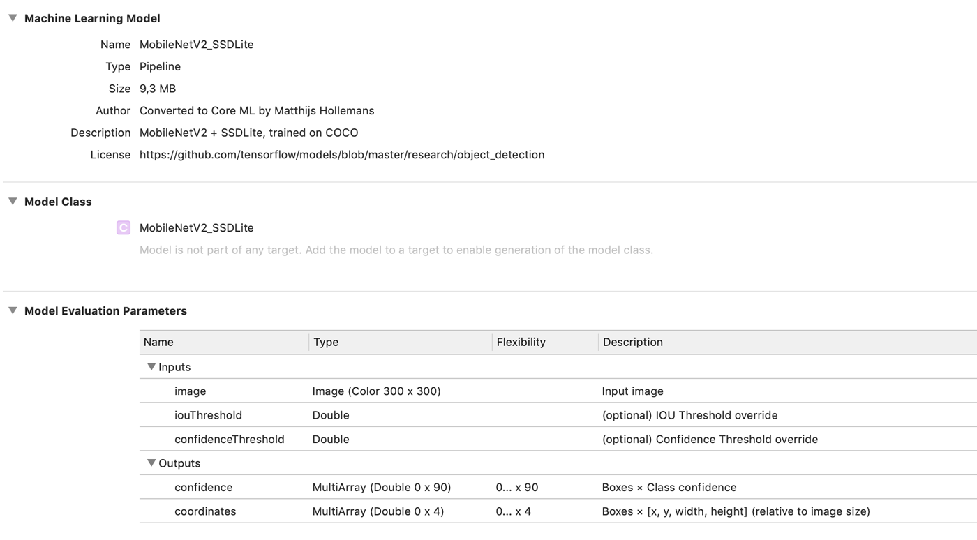
And there you have it: MobileNetV2_SSDLite.mlmodel is now a complete object detector model, including the logic that decodes the bounding box coordinates and non-maximum suppression.
When you open the mlmodel file in Xcode, it now looks like this:
You can find the full conversion script, ssdlite.py, in the repo for the book.
Using the model in an app
This is as easy as it gets. First create the VNCoreMLModel instance:
let coreMLModel = MobileNetV2_SSDLite()

lazy var visionModel: VNCoreMLModel = {
  do {
    return try VNCoreMLModel(for: coreMLModel.model)
  } catch {
    fatalError("Failed to create VNCoreMLModel: \(error)")
  }
}()
Then create the VNCoreMLRequest object:
lazy var visionRequest: VNCoreMLRequest = {
  let request = VNCoreMLRequest(model: visionModel, completionHandler: {
    [weak self] request, error in
    if let results = request.results as? [VNRecognizedObjectObservation] {
      /* do something with the results here */
    }
  })
  request.imageCropAndScaleOption = .scaleFill
  return request
}()
When you’re ready to make a prediction, create a VNImageRequestHandler:
let handler = VNImageRequestHandler(cvPixelBuffer: pixelBuffer)
do {
  try handler.perform([self.visionRequest])
} catch {
  print("Failed to perform Vision request: \(error)")
}
Inside the completion handler for the VNCoreMLRequest you get the results as an array of VNRecognizedObjectObservation objects.
There is one such object for every detected object in the image. The observation object contains a property labels with the classification scores for the class labels, and a property boundingBox with the coordinates of the bounding box rectangle.
And that’s really all there is to it! All the math and post-processing is done inside the Core ML model already. All you need to do is make the request and look at the VNRecognizedObjectObservation result objects.
Note: The IOU and confidence thresholds are optional but it doesn’t look like you can set these with Vision. There is no API in Vision that lets you pass in any input values except for a single image. Of course, if you use Core ML directly you can set these thresholds, but you’ll also need to read the bounding box coordinates and class scores from the MLMultiArray by yourself, so you lose the convenience of having VNRecognizedObjectObservation objects.
If you want to draw the bounding box rectangles, there are a few things to keep in mind:
- The
imageCropAndScaleOptionis important because it determines how the original input image is transformed before it goes into the Core ML model. You will need to apply the inverse transformation to the bounding box coordinates. - The predicted bounding box is in normalized image coordinates, which go from 0 to 1. You will need to scale them up to the size at which you’re displaying the image.
- The origin of the bounding box coordinates is in the lower-left corner. That’s just how Vision likes to do things.
The repo for the book contains a demo app that runs the MobileNetV2+SSDLite model on the live camera feed. Here it is in action in my kitchen:

By the way, recall that we stored the names of the class labels inside the model’s metadata. You can read those label names using the following code:
guard let userDefined = coreMLModel.model.modelDescription
        .metadata[MLModelMetadataKey.creatorDefinedKey] as? [String: String],
    let allLabels = userDefined["classes"] else {
  fatalError("Missing metadata")
}

let labels = allLabels.components(separatedBy: ",")
The demo app uses this to assign a unique color to each class label when the model is first loaded.
Was it all worth it?
After having seen the effort it took to add the coordinate decoding and NMS into the Core ML model, you may be wondering if it’s really worth it — maybe doing this in a custom layer or with a bit of Swift code wasn’t such a bad idea after all?
The answer is: it depends.
If your goal is to get a model that runs as fast as possible, you’d have to measure the speed of the different implementations on different devices. That’s the only way to find out which approach is fastest.
The advantage of putting everything inside the same model is that it is much more convenient to use. It also lets Core ML choose the best hardware to run the model on. On the iPhone XS, this model runs on the Neural Engine. Currently that’s not possible if you use a custom layer.
It’s certainly possible that doing the decoding by yourself — using the Accelerate framework, for instance — ends up being a little faster than letting Core ML do it. With Core ML you have to use generic operations such as slice, permute and concat, while in your own code it’s just a matter of changing a pointer address.
But does it matter? Most of the time taken by this model is spent in the SSD neural network. Optimizing the coordinate decoding may not make any difference to the overall speed. Again, the only way to find out is to measure it!
* * *
How does the Core ML version of MobileNetV2+SSDLite compare to my optimized Metal version?
On all devices prior to the iPhone XS, the Metal version is much faster. Because my Metal implementation is hand-optimized, it can avoid all the overhead that is necessary for a general purpose framework such Core ML.
On the iPhone XS, the Metal version is still faster than Core ML — even when using the Neural Engine — but the speed difference is smaller.
To be honest, I had expected the Neural Engine to beat the pants off the GPU, just like it does for TinyYOLO. It turns out that MobileNetV2+SSDLite actually runs quite slowly on the Neural Engine.
TinyYOLO is much faster on the iPhone XS than SSDLite — which is interesting because on iPhones that do not have a Neural Engine it’s the other way around… MobileNetV2+SSDLite on the GPU is way faster than TinyYOLO.
I think this is because of the depthwise separable convolutions. The Neural Engine doesn’t really seem to get along very well with those.
* * *
I hope you enjoyed reading this (long!) chapter from my book Core ML Survival Guide. Don’t worry, most of the other chapters are much shorter! 😄
Still, there’s over 350 pages of Core ML tips and tricks packed into this guide — so if you’re looking to make the most out of Core ML, get the book!
First published on Monday, 17 December 2018.
If you liked this post, say hi on Twitter @mhollemans or LinkedIn.
Find the source code on my GitHub.
 New e-book: Code Your Own Synth Plug-Ins With C++ and JUCE
Interested in how computers make sound? Learn the fundamentals of audio programming by building a fully-featured software synthesizer plug-in, with every step explained in detail. Not too much math, lots of in-depth information! Get the book at Leanpub.com