The “hello world” of neural networks

Neural networks — also known as “deep learning” — are hot!

And now iOS 10 and macOS 10.12 come with the BNNS framework, or Basic Neural Network Subroutines, that lets you put neural networks into your own apps.

BNNS runs on the CPU and is heavily optimized to be as fast as possible. There is also a version of these routines that use Metal and the GPU (part of the Metal Performance Shaders framework).

In this post I’ll show you how to get a really basic neural network up and running with BNNS.

We’re going to build a neural network that can compute the XOR function. If your binary logic is a little rusty, this is what XOR (exclusive-or) computes:

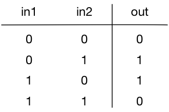
In other words, the result of XOR is 1 (true) if one of the inputs is 1 (true) but the other is 0 (false). If both inputs are false or both inputs are true, then their XOR is false.

In most programming languages you compute the XOR like so:

a = 1
b = 0
c = a ^ b   // answer: 1

In this post I’ll show you how to use a neural network to compute the XOR of two numbers. This may seem a little silly, since it will be a lot slower than just doing it using the binary ^ operator. However, it was not possible to compute XOR with perceptrons, an early type of neural network, and this eventually led to the first AI winter. So the idea is not completely ridiculous…

The neural network that we’re going to build looks like this:

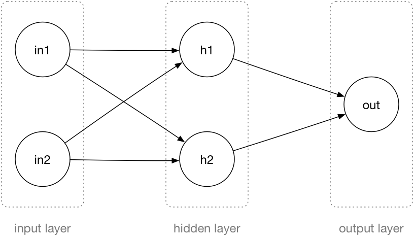
A neural network consists of layers, and each layer has neurons. This network has three layers: an input layer, a hidden layer, and an output layer.

The input to this neural network is two binary numbers that you put in the in1 and in2 neurons.

These two inputs are connected to the neurons in the hidden layer, h1 and h2. The hidden layer performs some computation and passes the result to the output layer neuron out. This also does a computation and then outputs a 0 or a 1.

Notice that the neurons in the input layer don’t actually do anything, they are just placeholders for the input value. Only the neurons in the hidden layer and the output layer perform computations.

As you can see in the illustration, all the neurons from the input layer are connected to all the neurons in the hidden layer. Likewise, both neurons from the hidden layer are connected to the output layer. These kinds of layers are called fully-connected because every neuron is connected to every neuron in the next layer.

Each connection between two neurons has a weight, which is just a number:

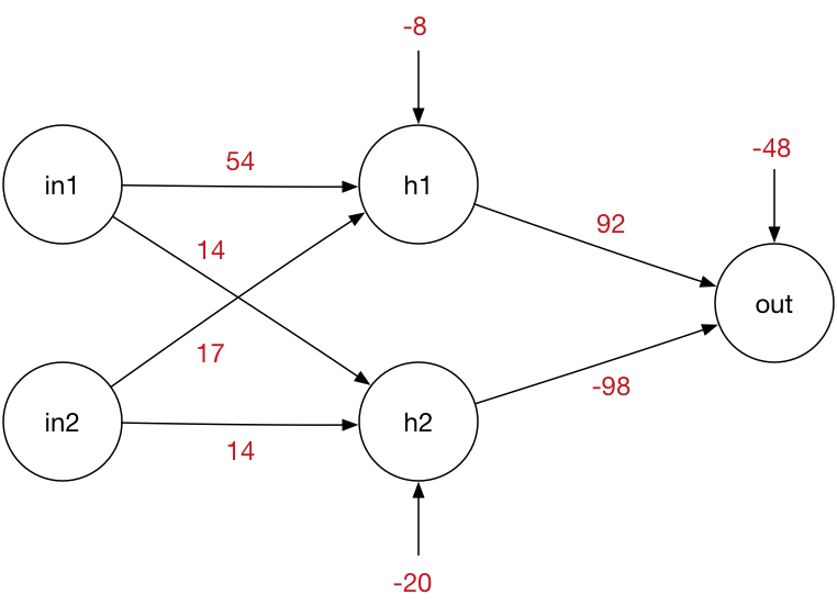
These weights form the brain of the network: the particular values that you see in the image describe the XOR function. If you were to use different numbers, then the network will no longer compute the XOR of the two input values but some other function.

Also notice the extra number going into each neuron. This is called the bias.

The neurons in the hidden layer perform the following computation:

h1 = sigmoid(in1 * w1 + in2 * w2 + b1)
h2 = sigmoid(in1 * w3 + in2 * w4 + b2)

where w1, w2, w3, w4 are the weights and b1 and b2 are the bias values. If we fill in those weights and biases with the numbers from the illustration, the equations become:

h1 = sigmoid(in1 * 54 + in2 * 17 - 8)
h2 = sigmoid(in1 * 14 + in2 * 14 - 20)

sigmoid() is a mathematical function that looks like this (in pseudocode):

func sigmoid(x) {
  return 1 / (1 + exp(-x))
}

This is also known as the activation function of the network. There are several different activation functions and BNNS supports the most common ones.

It doesn’t really matter so much what this activation function does, as long as it turns the linear equation in1 * w1 + in2 * w2 + b1 into something that is non-linear. This is important or the neural net wouldn’t be able to learn any interesting things — in other words, without this sigmoid thingie the network can’t perform the XOR function.

The graph of sigmoid() looks a bit like an “S”, which is where its name comes from (sigma is the Greek letter S):

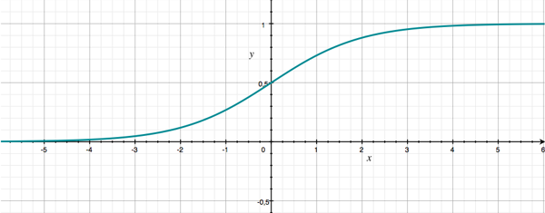
As you can see, the sigmoid takes in some number x and converts it into a value between 0 and 1. That is ideal for our purposes, since we’re dealing with binary numbers.

Because we want sigmoid() to output a nice binary 0 or 1, we have to make sure that the result from in1 * w1 + in2 * w2 + b1 is a large negative value (less than -5) or a large positive value (greater than +5). If x is too close to 0, sigmoid(x) will be some value between 0 and 1.

Let’s see what happens when we give the neural network some input.

If we set the input neurons to in1 = 0 and in2 = 0, then the values of the two hidden neurons h1 and h2 only depend on the biases because the terms with the weights become 0:

h1 = sigmoid(0 * 54 + 0 * 17 - 8)  = sigmoid(-8)  = 0.000335
h2 = sigmoid(0 * 14 + 0 * 14 - 20) = sigmoid(-20) = 0.000000

Both of these are pretty much zero.

For the input in1 = 0, in2 = 1, the hidden neurons will be:

h1 = sigmoid(0 * 54 + 1 * 17 - 8)  = sigmoid(9)  = 0.999876
h2 = sigmoid(0 * 14 + 1 * 14 - 20) = sigmoid(-6) = 0.002472

This time h1 has a value that is close to 1 while h2 is close to 0. Notice that these values never truly become 1.0 or 0.0 — the sigmoid function gets really close to these extremes but never quite reaches them.

In a similar manner you can compute the values of h1 and h2 for the other possible inputs (rounded off to 0 and 1):

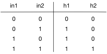
These are the possible values for the hidden neurons in this network for all possible inputs.

Since h1 and h2 are connected to the output neuron, again with their own weights and a new bias value, what the output neuron computes is this:

out = sigmoid(h1 * 92 + h2 * -98 - 48)

This pretty much does the same calculation as the h1 and h2 neurons, except that the weights and bias are different.

We want out to be close to 1 if h1 = 1 and h2 = 0 (see the above table). But in the other cases — if h1 and h2 are both 0 or are both 1 — out should be 0. Verify for yourself that the formula for out indeed computes this. Remember, sigmoid(large negative value) is 0 and sigmoid(large positive value) is 1.

OK, that’s the theory. Now let’s convert this to code.

First, we import the necessary libraries and then define two BNNSFilter objects:

#include <Accelerate/Accelerate.h>
#include <stdio.h>
#include <stdlib.h>
#include <string.h>

BNNSFilter hidden_layer;
BNNSFilter output_layer;

Note how BNNS does not use the term “layers” but calls them filters. You can think of these filters as sitting in between the layers of neurons:

This does the exact same thing but it’s a slightly different way of looking at the network. All the computations now happen inside these filters; the neurons are now just variables that hold a value.

The filters are created in the function create_network(). Here is the first part of that function:

bool create_network(void) {
    BNNSFilterParameters filter_params;
    bzero(&filter_params, sizeof(filter_params));
  
    BNNSActivation activation;
    bzero(&activation, sizeof(activation));
    activation.function = BNNSActivationFunctionSigmoid;
    
    float input_to_hidden_weights[] = { 54.0f, 14.0f, 17.0f, 14.0f };
    float input_to_hidden_bias[] = { -8.0f, -20.0f };
    float hidden_to_output_weights[] = { 92.0f, -98.0f };
    float hidden_to_output_bias[] = { -48.0f };    

We create a BNNSActivation object that describes the sigmoid function. We also define several arrays containing the weights and bias values.

Next up we describe the two filters:

    BNNSFullyConnectedLayerParameters input_to_hidden_params;
    bzero(&input_to_hidden_params, sizeof(input_to_hidden_params));
    input_to_hidden_params.in_size = 2;
    input_to_hidden_params.out_size = 2;
    input_to_hidden_params.activation = activation;
    input_to_hidden_params.weights.data = input_to_hidden_weights;
    input_to_hidden_params.weights.data_type = BNNSDataTypeFloat32;
    input_to_hidden_params.bias.data = input_to_hidden_bias;
    input_to_hidden_params.bias.data_type = BNNSDataTypeFloat32;
    
    BNNSFullyConnectedLayerParameters hidden_to_output_params;
    bzero(&hidden_to_output_params, sizeof(hidden_to_output_params));
    hidden_to_output_params.in_size = 2;
    hidden_to_output_params.out_size = 1;
    hidden_to_output_params.activation = activation;
    hidden_to_output_params.weights.data = hidden_to_output_weights;
    hidden_to_output_params.weights.data_type = BNNSDataTypeFloat32;
    hidden_to_output_params.bias.data = hidden_to_output_bias;
    hidden_to_output_params.bias.data_type = BNNSDataTypeFloat32;

Most of this is boilerplate to configure the filter objects. Of particular importance are in_size and out_size. The first filter has two inputs (in1 and in2) and two outputs (h1 and h2). The second filter has two inputs (h1 and h2) and one output (out). We also set the weights and bias values on the connections.

Next up we create the first filter that sits between the input neurons and the hidden neurons:

    BNNSVectorDescriptor input_desc;
    bzero(&input_desc, sizeof(input_desc));
    input_desc.size = 2;
    input_desc.data_type = BNNSDataTypeFloat32;
    
    BNNSVectorDescriptor hidden_desc;
    bzero(&hidden_desc, sizeof(hidden_desc));
    hidden_desc.size = 2;
    hidden_desc.data_type = BNNSDataTypeFloat32;
    
    hidden_layer = BNNSFilterCreateFullyConnectedLayer(&input_desc, 
                     &hidden_desc, &input_to_hidden_params, &filter_params);
    if (hidden_layer == NULL) {
        fprintf(stderr, "BNNSFilterCreateFullyConnectedLayer failed\n");
        return false;
    }    

And finally we create the second filter, between the hidden neurons and the output neuron:

    BNNSVectorDescriptor output_desc;
    bzero(&output_desc, sizeof(output_desc));
    output_desc.size = 1;
    output_desc.data_type = BNNSDataTypeFloat32;
    
    output_layer = BNNSFilterCreateFullyConnectedLayer(&hidden_desc, 
                    &output_desc, &hidden_to_output_params, &filter_params);
    if (output_layer == NULL) {
        fprintf(stderr, "BNNSFilterCreateFullyConnectedLayer failed\n");
        return false;
    }
    
    return true;
}

Even for a simple network such as this, create_network() is a fairly big function, but that’s mainly because you have to create all these descriptor objects to tell BNNS what your filters look like and what sort of data you’re going to send through the network.

Once you have created the network, you can use it to do inference. That is a fancy word for making predictions: you give the network some inputs and look at the output value.

float predict(float in1, float in2) {
    float input[]  = { in1, in2 };
    float hidden[] = { 0.0f, 0.0f };
    float output[] = { 0.0f };

    int status = BNNSFilterApply(hidden_layer, input, hidden);
    if (status != 0) {
        fprintf(stderr, "BNNSFilterApply failed on hidden_layer\n");
    }
    
    status = BNNSFilterApply(output_layer, hidden, output);
    if (status != 0) {
        fprintf(stderr, "BNNSFilterApply failed on output_layer\n");
    }

    printf("Predict %f, %f = %f\n", a, b, output[0]);
    return output[0];
}

The code in predict() is what computes the XOR function. The input, hidden, and output arrays hold the values of our neurons. We put the values of in1 and in2 into input and then call BNNSFilterApply() to fill in hidden and output.

Let’s put this all together into a program you can actually run:

int main(int argc, const char * argv[]) {
    if (create_network()) {
        printf("Making predictions for XOR gate:\n");
        
        predict(0, 0);
        predict(0, 1);
        predict(1, 0);
        predict(1, 1);
        
        destroy_network();
    }
    return 0;
}

The destroy_network() function cleans up by deallocating the filters when we’re done:

void destroy_network(void) {
    BNNSFilterDestroy(hidden_layer);
    BNNSFilterDestroy(output_layer);
}

The code that I’ve shown you here is the complete implementation of a neural network that acts like an XOR gate.

When you run the program, the output is:

Making predictions for XOR gate:
Predict 0.000000, 0.000000 = 0.000000
Predict 0.000000, 1.000000 = 1.000000
Predict 1.000000, 0.000000 = 1.000000
Predict 1.000000, 1.000000 = 0.000000
Program ended with exit code: 0

That looks like the correct answers to me!

You may be wondering where I got the magic numbers for the weights from. You can find these weights by training the network. Training is not done in this example program, since BNNS does not support training. Instead, I used a separate program to train the network and that gave me these weights.

I’m not going to go into much detail on how to train neural networks, but the basic idea is as follows:

1. Initialize the weights to small random values and the biases to zero.
2. Perform a forward pass through the network to make a prediction for your input data. This is what our predict() function does. This prediction will be wrong at first because the network has not learned anything yet.
3. Determine how wrong the prediction is. There are various ways to express this error, or “loss”, as some numeric quantity.
4. Perform a backward pass through the network and move the weights a little bit in the direction of the right answer. The next time you make a prediction for the same inputs, the answer will be a little more correct. BNNS has no facilities for doing such a backward pass, which is why you can’t use it for training.
5. Go to step 2 and repeat this several thousand times. With each iteration, the network will be a little less wrong.

Eventually, you end up with a set of weights that describe the XOR function — or any other thing you want the network to learn.

By the way, there’s nothing stopping you from using numbers other than 0 or 1 as the inputs. Here’s a plot I made of the decision boundary for this neural network:

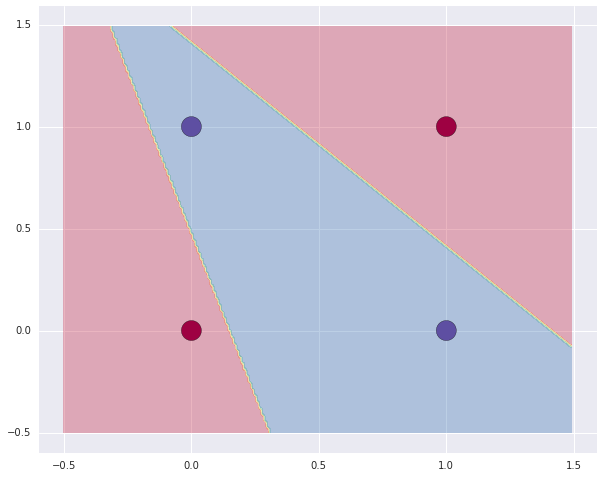
The blue area is where the neural network outputs 1, the red area is where it outputs 0.

You can find the full C source code in this gist, and the Swift version here.