Convolutional neural networks on the iPhone with VGGNet

I implemented the VGGNet architecture for image recognition on the iPhone, using the new convolutional neural network API from the Metal Performance Shaders framework.

In this post I explain how CNNs work and specifically how to get VGGNet running on your iPhone using Metal.

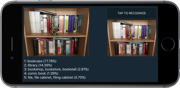
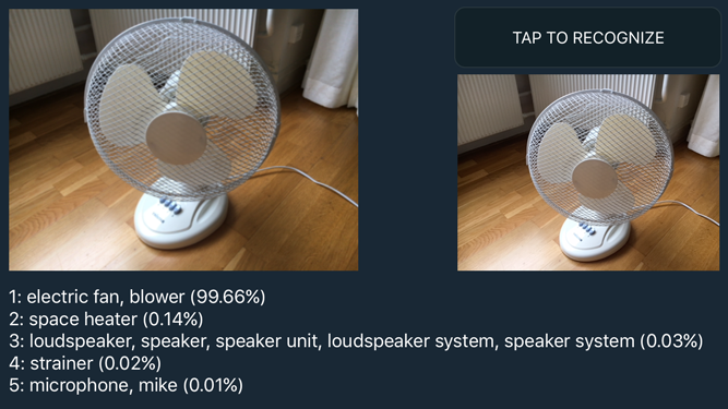
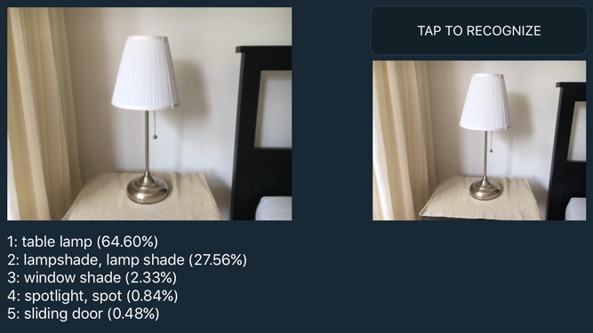
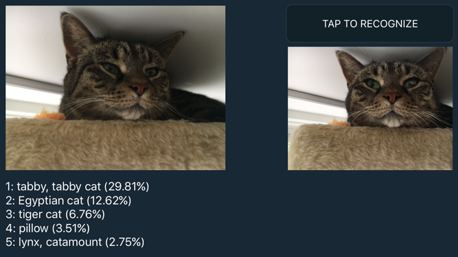
The demo app sends the video feed from the iPhone’s camera through the neural network to get the top-5 classification scores for whatever you’re looking at:

What is this all about?

VGGNet is a neural network that performed very well in the ImageNet Large Scale Visual Recognition Challenge (ILSVRC) in 2014. It scored first place on the image localization task and second place on the image classification task.

Localization is finding where in the image a certain object is, described by a bounding box. Classification is describing what the object in the image is. This predicts a category label, such as “tabby cat” or “bookcase”. We are going to be doing classification.

ImageNet is a huge database of images for academic researchers. Every year the people who run ImageNet host an image recognition competition. The goal is to write a piece of software — these days usually a neural network of some kind — that can correctly predict the category for a set of test images. Of course, the correct categories are known only to the contest organizers. (This keeps the neural networks honest.)

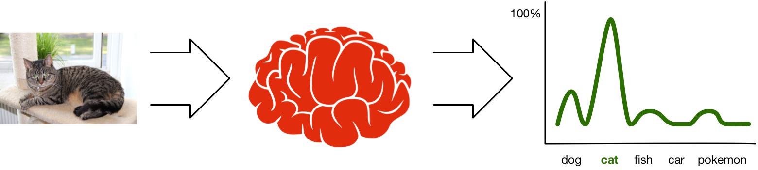
The images used in the competition are divided into 1000 different categories. Given a test image, the neural network will output a probability distribution for that image. This means it calculates a probability — a value between 0 and 1 — for each of those 1000 categories, then chooses the category with the highest probability.

If the neural network is very certain about a prediction, then its top choice has a high probability, such as 77.78% for the bookcase in the screenshot.

In the ImageNet classification challenge you actually get five chances to predict the right category, which is why the demo app shows the 5 highest probabilities the network computed. As you can see in the screenshot, the network also thinks the image could have been a library, bookshop, or comic book — but the probabilities indicate that it isn’t as confident about those choices.

The image recognizer with the smallest error wins the competition. Currently, the state of the art is about 3.5% wrong, which is actually better than human performance. (If you find this hard to believe, consider this: the data set contains about 200 different dog categories — can you tell all these species apart?)

The list of the 1000 category names looks like the following. Here are the first six categories:

n01440764 tench, Tinca tinca
n01443537 goldfish, Carassius auratus
n01484850 great white shark, white shark, man-eater, man-eating shark
n01491361 tiger shark, Galeocerdo cuvieri
n01494475 hammerhead, hammerhead shark
n01496331 electric ray, crampfish, numbfish, torpedo
...994 other categories omitted...

Apparently you also have to be good at recognizing fish when you enter this competition!

By the way, the identifier at the front is the WordNet ID. You can get a list of all the images for a category, say n01443537 goldfish, by going to the URL www.image-net.org/api/text/imagenet.synset.geturls?wnid=n01443537. To get a better idea of all the images in ImageNet, use image-net.org/explore.

Training the network

Participants in the ILSVRC competition can download a training set of about one million images. There are roughly 1000 images for each of the 1000 categories. The training set also includes the category names for these images — the so-called labels — because the network needs to know what each training image represents.

The idea is that you take these million or so training images and use them to train your neural network. This results in something called the learned parameters that describe what the neural network has learned.

Training these neural networks takes a lot of time! VGGNet apparently took 2-3 weeks to train on a computer with four NVIDIA Titan Black GPUs. Fortunately for us, once a neural network is trained we can simply take these learned parameters and use them in our own apps.

So what does it mean for a neural network to “learn” anything? Let’s say you want to train a network such as VGGNet to recognize faces of celebrities. During the training phase you use a dataset with a few hundred or thousand different photos of each celebrity (more is better!). Obviously, the network cannot remember each and every photo — that would take way too much memory.

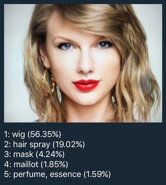
Instead, the training process somehow distills from these photos what it means to look like, say, Taylor Swift (celebrity of choice for iOS tutorial writers).

The neural network creates a kind of summary from all these training photos of Taytay: a bunch of numbers — also known as feature detectors — that capture what a “Taylor Swift” looks like.

Later, when you feed a new image of Taylor Swift into the network, one that you didn’t use for training, the feature detectors that react to the category “Taylor Swift” will be activated the most while the feature detectors for other celebrities stay silent. The network assigns a high probability to her category — something like 90% — and low probabilities to all the other celebs.

Now what happens when you give the network a photo of someone who was not in the training set, let’s say this person? The network will still try to match this photo to one of the categories it knows about. In this case, it might conclude that this other person also matches the criteria for “looking like Taylor Swift” but with a lower confidence score, say only 60% probability.

So in that sense, what the network really learns isn’t so much what Taylor looks like, but whatever it is that distinguishes her photos from the other people you trained on.

Neural networks aren’t magic: they can only recognize things you trained them to recognize. Since the VGGNet we’re using was trained on ImageNet, it’s really good at distinguishing between different breeds of dogs, different types of fish, and so on. But there are plenty of objects that it doesn’t know about. (Apparently VGGNet wasn’t trained on photos of Taylor. Or does it know something we don’t!?)

OK, so the network learns things and we call this the “learned parameters”. What exactly are those then? It’s less fancy than you might think: the learned parameters are nothing more than the weights between the various connections in the neural network. I’ll tell you all about that in the next section.

Deep learning with convolutional neural networks

You can think of a neural network as a pipeline: data goes in one end, it is transformed in different stages, and finally comes out at the other end in a different shape.

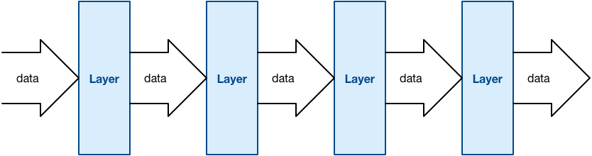
The things that perform the transformations are called the layers. (Apple’s other neural networks framework, BNNS, calls them filters but that’s a little confusing as the term “filter” is also used to describe convolution operations.)

The VGGNet architecture looks like this, it has 21 layers:

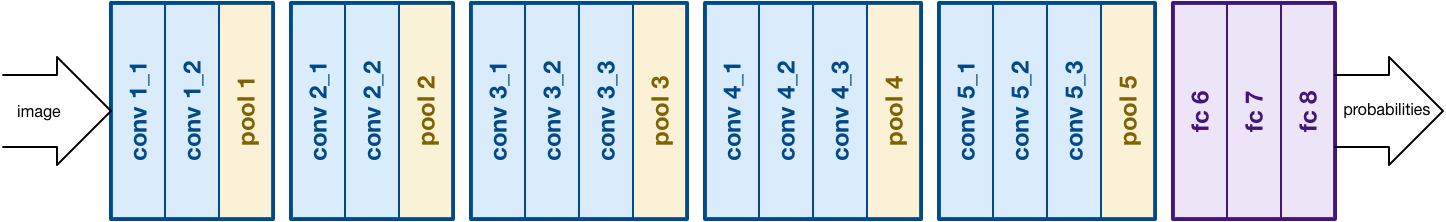
A typical pattern you see in CNNs is that two or three convolutional layers are followed by a pooling layer. In VGGNet there are 5 such groups. At the end of the network are three fully-connected (or “fc”) layers.

You can see where the term “deep learning” comes from: this is a deep network because it has many layers. More recent networks even have 100+ layers! I will explain how all these different layers work in the coming sections.

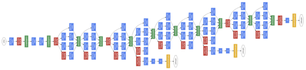
Note: What you see in the picture above isn’t the only way to structure a conv net — in fact, many other architectures exist. I chose VGGNet because it has a very straightforward structure, which makes it easier to explain. Here’s a little taster of what Google’s Inception network looks like:

To use VGGNet you put an image into the first layer, conv1_1. This layer applies a transformation to the image’s pixels and sends it to the next layer, conv1_2. That also transforms the data and sends it to pool1, and so on, until the image reaches the last layer, fc8.

The very last layer applies the softmax function to the data in order to output a probability distribution. It’s not very important to understand the math — just know that you end up with an array of 1000 floating-point values, each corresponding to one of the possible image categories. The array element with the largest value has the highest probability, and is therefore the category that the network predicts.

By the way, “VGG” stands for the Visual Geometry Group from the University of Oxford. They are the people who came up with this particular neural network and who trained it on the ImageNet dataset. For the full lowdown on VGGNet you can read the original research paper:

Very Deep Convolutional Networks for Large-Scale Image Recognition
K. Simonyan, A. Zisserman
arXiv:1409.1556

Now let’s look at these layers in more detail.

Fully-connected layers

The classical type of neural network layer is the fully-connected layer, or “FC” layer:

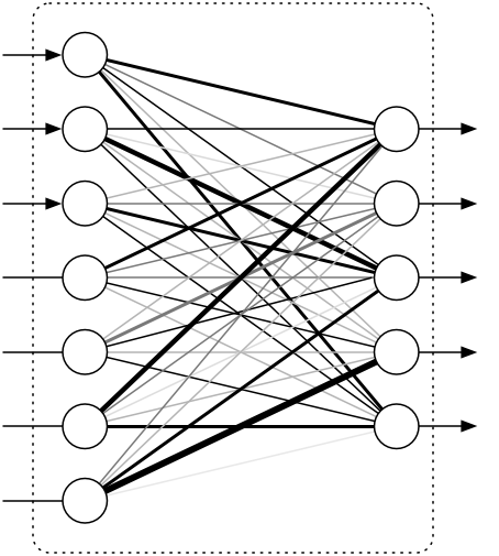
The input to this layer is a vector of numbers. Each of the inputs is connected to every one of the outputs — hence the term “fully connected”. These connections have weights that determine how important they are (illustrated by thick and thin lines in the picture). The output is also a vector of numbers.

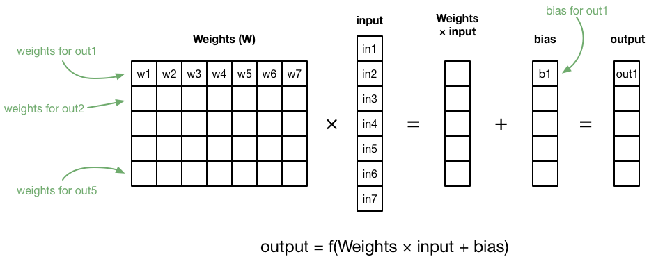
As I said, each layer transforms the data. The computation that is performed by this layer is as follows. For each output element, we take a weighted sum of all the input elements and add a so-called bias term:

in1*w1 + in2*w2 + in3*w3 + ... + in7*w7 + b1

This is similar to the equation of a line that you learned in high school: y = a x + b where a is the slope of the line and b is the y-intercept, except there is a separate slope — the weight — for each input element. In other words, what you’re computing here is a linear function across all the inputs (in many dimensions).

Since linear functions aren’t very exciting, we also apply an activation function to the weighted sum:

out1 = f(in1*w1 + in2*w2 + in3*w3 + ... + in7*w7 + b1)

The function f() can be anything you want, as long as it introduces some kind of non-linearity, otherwise the network can’t learn anything interesting.

The classical activation function is the sigmoid function f(x) = 1/(1 + exp(-x)), but in most convolutional networks people use the rectified linear unit or ReLU. That sounds very fancy but it’s just f(x) = max(0, x); it only lets inputs through that are greater than 0. One reason ReLUs are popular these days is that they’re a lot faster to compute than sigmoids.

Fun math fact: If you put the weights into a matrix, and the inputs and biases into vectors, you can actually compute the entire fully-connected layer with a single statement.

The important thing about the fully-connected layer is the weights for the connections. These represent what the network has learned. When you train the network, you continually adjust those weights up and down until the network does what you want it to. When people talk about the “learned parameters” of a neural network, they are talking about these weights.

So that’s a fully-connected layer. It’s pretty simple, just a bunch of inputs that take data from a previous layer and a bunch of outputs that send data to the next layer. Inside the layer, the data gets transformed by the weighted sums and the activation function.

Unfortunately, FC layers have a bit of a downside. The example layer had 7 inputs and 5 outputs, so it has 7×5 = 35 connections between them and thus requires 35 weights (and 5 biases, one for each output). Now let’s look at VGGNet: the output of the pool5 layer is 25,088 values. These become the inputs of the fc6 layer, which itself has 4096 outputs. The number of connections in fc6 is therefore 25,088 × 4096 = 102.760.448. That’s a lot!

In fact, the total number of parameters in VGGNet is about 130 million. This means the learned parameters for VGGNet largely consist of the weights for this one layer!

Convolutional layers

The real power of these deep learning networks, especially for image recognition, comes from convolutional layers.

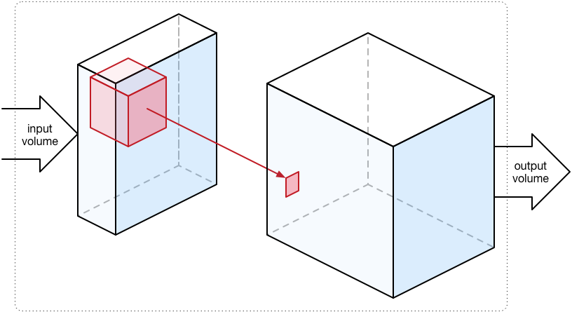
With a fully-connected layer, the input and output are one-dimensional vectors of numbers. However, a convolutional layer works on three-dimensional volumes of data (also called tensors). The output usually has the same width and height as the input volume but a larger depth.

You can think of an image as a three dimensional “cube”. The width and height are as usual, but each of the RGB components gets its own plane:

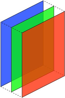
This is the input we give to VGGNet: a 3D tensor describing the image that we want to classify. In Metal, that tensor is described by an MPSImage object. All the data that flows into the network, between each of the layers, and out of the network at the other end is represented by MPSImage objects.

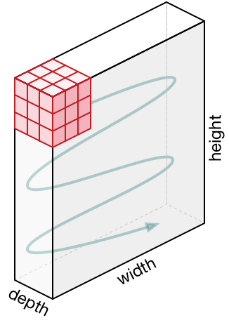
The convolutional layer runs a convolution kernel over the 3D input volume. This is exactly the same thing as the convolutions used in image processing, but in multiple dimensions. The convolution kernel is also a 3D volume but typically a lot smaller than the input. In VGGNet they are always 3×3 pixels wide and tall, and just as deep as the input volume (in the below illustration, the input volume is 3 deep, so the kernel is 3×3×3).

We slide this cube that is the convolution kernel across the entire input volume, from left to right, top to bottom. Think of this as an eye scanning over the input image where it only looks at a 3×3 region at a time.

At each position we simply add up the 27 input elements inside this cube and write the sum to the output. Just like with an FC layer, we multiply the inputs with the weights:

in1*w1 + in2*w2 + in3*w3 + ... + i27*w27 + b

Here the weights belong to the convolution kernel. If a kernel is 3×3×3, it has 27 weights. Recall that in a fully-connected layer, a weight described the strength of the connection between an input and an output. In a convolutional layer, the weights describe what this kernel has learned so far — in particular, what features it has learned to detect. So for a convolutional layer, the learned parameters are the weights for its convolutional kernels.

The value that is written to the output volume is then:

out1 = relu(in1*w1 + in2*w2 + in3*w3 + ... + i27*w27 + b)

where relu() is the activation function of choice for the convolutional layer. If out1 is less than 0, the ReLU will make it 0. That’s all it does.

Because we slide the convolution kernel across the input volume it gets applied to each input element in turn. If the input image is 224×224 RGB — a 224×224×3 volume — then running the convolution kernel across that image results in a 224×224×1 output volume. Notice that the output depth is now 1, since the result of each convolution operation is a single value. So the width and height of the data stay the same but the depth gets squashed into a single layer.

Each convolutional layer actually has more than one convolution kernel. The first layers in VGGNet have 64 kernels, the layers at the end have 512. These convolutions are performed one after the other (on the original input data) and the results are stacked in the output of the layer, making this a 3D volume too.

For example, the first layer conv1_1 receives a 224×224×3 input volume. It has 64 convolution kernels, so its output volume is 224×224×64.

This is what happens to the volumes as they go through the VGGNet network:

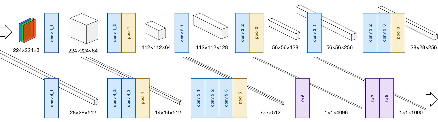
Notice how sometimes the width and height of the volumes gets reduced. This is done by a pooling or subsampling layer. You use pooling layers to cut down on the amount of data going through the network, but also to focus the network on the important bits. VGGNet uses so-called max pooling layers. Out of every 2×2 grid of input values, the pooling layer only keeps the one with the highest activation, i.e. it picks the one who shouts the loudest. ;–) There are no parameters to learn for these pooling layers, so that’s easy.

The MPSImage you insert into the network represents an actual image, usually a photo. Each plane in this first 224×224×3 input volume is a color channel. The first convolutional layer conv1_1 transforms this image into a 224×224×64 volume. As you go through the network, this volume becomes smaller in width and height but larger in depth. The very last pooling layer, pool5, outputs a 7×7×512 volume. So we’ve gone from a 224×224 RGB image to something that is only 7×7 “pixels” in size, but in depth we’ve grown from 3 to 512 planes of data.

* * *

Convolutional layers are great for image recognition because they scan the input much like a human eye does. Just as with the fully-connected layer, what we learn is weights — but here these weights are inside the convolution kernels. Since the kernels are small, 3×3 for VGGNet, a convolutional layer has many many fewer weights than a fully-connected layer.

For example, conv5_1 is one of the big conv layers in the network. Its input volume is 512 deep, so per kernel it requires 3×3×512 weights. And we have 512 of those kernels in this layer, so that is 3×3×512×512 = 2,359,296 weights in total (plus a handful of bias values). That’s 2.36 million weights, still nothing to sneeze at, but tiny compared to 100+ million weights for a big fully-connected layer such as fc6.

The really cool thing is that these convolution kernels learn to detect features in the input image. You simply initialize them with small random numbers, then train the network across many images, and the kernels will automatically learn what is interesting in the image. The early conv layers learn very low-level abstract features — where edges are, where color blobs are, etc — but the deeper into the network you go, the more specific these features get.

Here is a great video that demonstrates what some of these convolution kernels learn. For example, there is one that has learned to recognize when and where a photo contains a human face. Cool stuff!

Inference, or how to use a conv net

As I mentioned before, VGGNet took several weeks to train. This is obviously not something you want to do on the iPhone but on a powerful dedicated machine — or even cluster of such machines. Metal doesn’t even provide an API for training a neural network on the iPhone.

The only thing you can do with a neural net on the iPhone is inference, a fancy word for making predictions.

In our app, we’ll take an input image — either from the camera or by loading a JPG or PNG file — and give it to the neural network. The GPU will then perform all the computations, making the image data flow from layer to layer, transforming it in this process from a 224×224×3 volume into a vector of 1000 probabilities. Then we take the top 5 of those predictions and display them on the screen.

Rockin’ out with Metal Performance Shaders

OK, let’s put all this theory into practice. As of iOS 10, the Metal Performance Shaders framework includes support for convolutional neural networks.

Why Metal? The answer is that CNNs can be efficiently implemented on the GPU. It takes a billion or so computations to send a single image through the network, so we need all the computing power we can get!

The learned parameters

I’ve mentioned that the learned parameters of VGGNet consist of the kernel weights from the convolutional layers and the connection weights from the fully-connected layers (including bias values). Pool layers have no parameters.

For this project, we’re using the parameters that VGGNet has learned on the ImageNet dataset from the ILSVRC-2014 competition. These parameters are freely downloadable from the Caffe Model Zoo. This is a 553 MB file that contains everything VGGNet has learned when it was trained on the ImageNet dataset.

Caffe, by the way, is a popular tool for making — and training — neural nets. We’re not going to use Caffe, but the VGGNet download happens to be in .caffemodel format.

We can’t use the .caffemodel file directly, so I hacked together a Python script that reads this file and converts it to a big blob of raw floating point values. This file is called parameters.data and is inserted into the app bundle during compile time.

That’s right: when you include VGGNet into your app, the app bundle grows by 550+ MB thanks to those learned parameters. w00t!

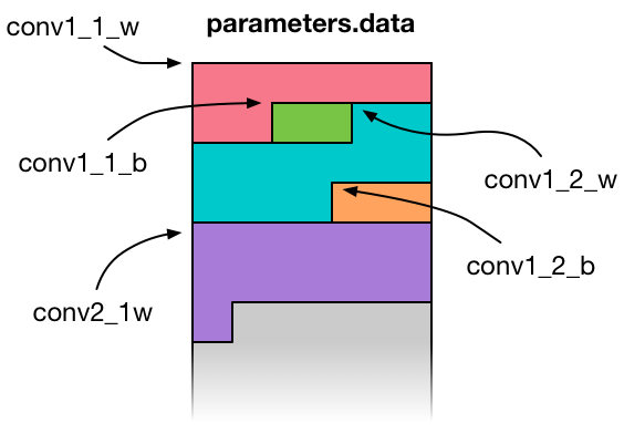
I’ve created a class VGGNetData that encapsulates all this. This class has properties for each layer’s weights and bias arrays:

class VGGNetData {
  var conv1_1_w: UnsafeMutablePointer<Float> { return ptr + 0 }
  var conv1_1_b: UnsafeMutablePointer<Float> { return ptr + 1728 }
  var conv1_2_w: UnsafeMutablePointer<Float> { return ptr + 1792 }
  var conv1_2_b: UnsafeMutablePointer<Float> { return ptr + 38656 }
  var conv2_1_w: UnsafeMutablePointer<Float> { return ptr + 38720 }
  ...
  var fc8_w: UnsafeMutablePointer<Float> { return ptr + 134260544 }
  var fc8_b: UnsafeMutablePointer<Float> { return ptr + 138356544 }

Here, ptr is a pointer to the start of the big data blob in memory, and conv1_1_w, conv1_1_b, conv1_2_w, and so on return pointers to their respective data arrays inside that big blob (w for weights, b for bias values).

When the app starts up, we use VGGNetData to load parameters.data into memory in one go, then we copy the learned parameters into the MPSCNNConvolution and MPSCNNFullyConnected objects for the layers, and immediately unload parameters.data again. You don’t want such a big file sticking around in memory.

Creating the network

Most of the code lives in the VGGNet class. This has a number of properties that represent the layers from this network:

let conv1_1: MPSCNNConvolution
let conv1_2: MPSCNNConvolution
let pool1  : MPSCNNPoolingMax

let conv2_1: MPSCNNConvolution
let conv2_2: MPSCNNConvolution
let pool2  : MPSCNNPoolingMax

let conv3_1: MPSCNNConvolution
let conv3_2: MPSCNNConvolution
let conv3_3: MPSCNNConvolution
let pool3  : MPSCNNPoolingMax 

let conv4_1: MPSCNNConvolution
let conv4_2: MPSCNNConvolution
let conv4_3: MPSCNNConvolution
let pool4  : MPSCNNPoolingMax

let conv5_1: MPSCNNConvolution
let conv5_2: MPSCNNConvolution
let conv5_3: MPSCNNConvolution
let pool5  : MPSCNNPoolingMax

let fc6: MPSCNNFullyConnected
let fc7: MPSCNNFullyConnected
let fc8: MPSCNNFullyConnected

As you can guess from the names, MPSCNNConvolution, MPSCNNPoolingMax, and MPSCNNFullyConnected are the Metal classes for the different types of layers.

VGGNet also has a list of MPSImageDescriptor objects that describe the shapes of the data volumes that go into and out of the layers:

let input_id  = MPSImageDescriptor(channelFormat: .float16, 
                       width: 224, height: 224, featureChannels: 3)
let conv1_id  = MPSImageDescriptor(channelFormat: .float16,
                       width: 224, height: 224, featureChannels: 64)
let pool1_id  = MPSImageDescriptor(channelFormat: .float16,
                       width: 112, height: 112, featureChannels: 64)
let conv2_id  = MPSImageDescriptor(channelFormat: .float16,
                       width: 112, height: 112, featureChannels: 128)
let pool2_id  = MPSImageDescriptor(channelFormat: .float16,
                       width:  56, height:  56, featureChannels: 128)
let conv3_id  = MPSImageDescriptor(channelFormat: .float16,
                       width:  56, height:  56, featureChannels: 256)
let pool3_id  = MPSImageDescriptor(channelFormat: .float16,
                       width:  28, height:  28, featureChannels: 256)
let conv4_id  = MPSImageDescriptor(channelFormat: .float16,
                       width:  28, height:  28, featureChannels: 512)
let pool4_id  = MPSImageDescriptor(channelFormat: .float16,
                       width:  14, height:  14, featureChannels: 512)
let conv5_id  = MPSImageDescriptor(channelFormat: .float16,
                       width:  14, height:  14, featureChannels: 512)
let pool5_id  = MPSImageDescriptor(channelFormat: .float16,
                       width:   7, height:   7, featureChannels: 512)
let fc_id     = MPSImageDescriptor(channelFormat: .float16,
                       width:   1, height:   1, featureChannels: 4096)
let output_id = MPSImageDescriptor(channelFormat: .float16,
                       width:   1, height:   1, featureChannels: 1000)

Remember that picture I sketched where the data volumes go into and out of the VGGNet layers? That is what these MPSImageDescriptor objects are describing. featureChannels is the term Metal uses for the depth of the volumes. It’s a bit tedious that you have to write it out this way, but believe me, for VGGNet it’s a lot simpler than for some other neural nets (<cough> Inception).

In VGGNet’s init() method, we create the layer objects:

conv1_1 = makeConv(device: device, inDepth:   3, outDepth:  64, 
                   weights: blob.conv1_1_w, bias: blob.conv1_1_b)
conv1_2 = makeConv(device: device, inDepth:  64, outDepth:  64, 
                   weights: blob.conv1_2_w, bias: blob.conv1_2_b)
pool1   = makePool(device: device)

conv2_1 = makeConv(device: device, inDepth:  64, outDepth: 128, 
                   weights: blob.conv2_1_w, bias: blob.conv2_1_b)
conv2_2 = makeConv(device: device, inDepth: 128, outDepth: 128, 
                   weights: blob.conv2_2_w, bias: blob.conv2_2_b)

//...and so on...

fc6 = makeFC(device: device, inExtent: 7, inDepth:  512, fanOut: 4096,
             weights: blob.fc6_w, bias: blob.fc6_b)
fc7 = makeFC(device: device, inExtent: 1, inDepth: 4096, fanOut: 4096,
             weights: blob.fc7_w, bias: blob.fc7_b)
fc8 = makeFC(device: device, inExtent: 1, inDepth: 4096, fanOut: 1000,
             weights: blob.fc8_w, bias: blob.fc8_b, withRelu: false)

Notice how we’re using blob.conv1_1_w and so on to pass the weights to the layers, where blob is an instance of VGGNetData.

The real work happens in the convenience functions makeConv(), makePool(), and makeFC(). For example, makeConv() looks like this:

private func makeConv(device: MTLDevice,
                      inDepth: Int,
                      outDepth: Int,
                      weights: UnsafePointer<Float>,
                      bias: UnsafePointer<Float>) -> MPSCNNConvolution {

  let relu = MPSCNNNeuronReLU(device: device, a: 0)

  let desc = MPSCNNConvolutionDescriptor(kernelWidth: 3,
                                         kernelHeight: 3,
                                         inputFeatureChannels: inDepth,
                                         outputFeatureChannels: outDepth,
                                         neuronFilter: relu)
  desc.strideInPixelsX = 1
  desc.strideInPixelsY = 1

  let conv = MPSCNNConvolution(device: device,
                               convolutionDescriptor: desc,
                               kernelWeights: weights,
                               biasTerms: bias,
                               flags: MPSCNNConvolutionFlags.none)
  return conv
}

To create a convolutional layer, you need a MPSCNNConvolutionDescriptor object. The code here tells Metal that we want to use a 3×3 convolution kernel with stride 1, and to apply a ReLU activation function after the convolution. The configuration of all conv layers in VGGNet is the same, except for the input depth, output depth, and the learned parameters (weights and bias).

The code for makePool() and makeFC() is very similar, so I won’t show it here.

And that’s how the network gets created. You just put together a series of MPSCNNConvolution, MPSCNNPoolingMax, and MPSCNNFullyConnected instances.

Making a prediction

All right, now that the network is set up we can use it to perform inference. The workflow is as follows:

1. Load an image from a JPG or PNG file, or grab a frame from the iPhone’s camera, and put it into an MPSImage object.
2. Do some preprocessing to make sure it is in the format that the network expects (see next section).
3. Put the processed image into the first layer, conv1_1. This results in a new MPSImage. Actually, we use MPSTemporaryImage for this, which is more efficient.
4. Take that MPSTemporaryImage and put it into conv1_2. This gives us another MPSTemporaryImage.
5. Take the output image from conv1_2 and put it into pool1.
6. Take the output from pool1 and put it into conv2_1.
7. Take the output from conv2_1 and put it into conv2_2.
8. …and so on until we’ve done all the layers…
9. Take the output image from fc8 and apply the softmax function to it.

When all that is done, convert the final MPSImage into a Swift [Float] array. Then look up the category labels and place them on the screen.

In code, steps 3 – 9 look like this:

let conv1_1_img = MPSTemporaryImage(commandBuffer: commandBuffer, 
                                    imageDescriptor: conv1_id)
conv1_1.encode(commandBuffer: commandBuffer, sourceImage: img2, 
               destinationImage: conv1_1_img)

let conv1_2_img = MPSTemporaryImage(commandBuffer: commandBuffer, 
                                    imageDescriptor: conv1_id)
conv1_2.encode(commandBuffer: commandBuffer, sourceImage: conv1_1_img, 
               destinationImage: conv1_2_img)

let pool1_img = MPSTemporaryImage(commandBuffer: commandBuffer, 
                                  imageDescriptor: pool1_id)
pool1.encode(commandBuffer: commandBuffer, sourceImage: conv1_2_img, 
             destinationImage: pool1_img)

let conv2_1_img = MPSTemporaryImage(commandBuffer: commandBuffer, 
                                    imageDescriptor: conv2_id)
conv2_1.encode(commandBuffer: commandBuffer, sourceImage: pool1_img, 
               destinationImage: conv2_1_img)

//...and so on...

let fc8_img = MPSTemporaryImage(commandBuffer: commandBuffer, 
                                imageDescriptor: output_id)
fc8.encode(commandBuffer: commandBuffer, sourceImage: fc7_img, 
           destinationImage: fc8_img)

softmax.encode(commandBuffer: commandBuffer, sourceImage: fc8_img, 
               destinationImage: outputImage)

For every layer you grab a new MPSTemporaryImage, then call encode() on the layer object. You simply repeat this for all of the layers until the very end. A bit tedious, but that’s how it works.

After the softmax finishes, outputImage contains a vector of 1000 floating point numbers for the probabilities of each of our 1000 possible image categories. I’ll explain in a minute how we convert this to actual category labels, but first I have to tell you about another important topic…

Preprocessing the image

We have a JPG or PNG image loaded from a file, or a video frame that we grabbed from the camera, and we need to feed that into the neural network in order to get a prediction. However, the neural net has some requirements:

The image must be an MPSImage object

You can make an MPSImage from a regular Metal MTLTexture object. For JPG and PNG images, we simply use the MTKTextureLoader to get such a texture. For a photo from the iPhone’s camera it’s a bit more involved: we use a combination of the AVFoundation and CoreVideo frameworks to create the texture. See the file VideoCapture.swift for more details.

The MPSImage needs to be in .float16 format, but ours is most likely .unorm8

When you load a JPG or PNG file, or grab a frame from the camera, you’ll get an image where the R, G, B components of each pixel are 8-bit unsigned numbers. One pixel is 32 bits or 4 bytes, one byte per color channel ranging between 0 and 255. When you load this image into a Metal texture, it will typically have a pixel format such as MTLPixelFormatBGRA8Unorm (MPSImage calls this .unorm8).

This isn’t actually a big deal: if we put a .unorm8 image into the neural network, Metal will automatically convert it to .float16. However, there is a wrinkle: after converting to .float16, the colors in the image are now in the range 0 – 1 but VGGNet expects colors to go from 0 to 255. So we need to scale the colors up again by a factor of 255.

The input depth must be 3

The depth of conv1_1’s input volume is 3 because it expects three color channels (RGB). However, the MTLTexture most likely contains 4 channels (RGB + alpha). So when we create the MPSImage object, we tell it to only use 3 featureChannels.

The image needs to be 224×224 pixels

This is the width and height of the input volume that layer conv1_1 expects. It turns out that Metal has a convenient filter for this: MPSImageLanczosScale. Before we give the MPSImage to conv1_1, we first send it through a MPSImageLanczosScale filter to shrink it down.

The pixels must be in BGR order

The Caffe tool that was used to train VGGNet uses a BGR pixel order instead of the more usual RGB, and therefore so must we. Pictures coming from the camera are already in BGR order — however, the above resizing operation makes it RGB again, and so we must flip the R and B channels anyway.

We need to subtract the “mean RGB” value from each pixel

When VGGNet was trained on the ImageNet data, they computed the average values for R, G, and B across the training set. Before training on an image, these average values were subtracted from the image’s pixels. That gives an input image that is “zero-centered” — if you now take the average value of all the pixels in the image, you end up with 0. This has certain desireable mathematical properties.

For us that means we need to do the same for our images or they won’t make sense to the network. For VGGNet, from the red color component you subtract 123.68, from green you subtract 116.779, and from blue 103.939. (Notice that now the range of our input pixels is no longer 0 – 255 but approximately -128 to +128.)

We could do this on the CPU: first get the image’s raw bytes, then convert these UInt8 values to Floats (using Accelerate framework and vImage, for example). Then subtract the mean values from these floats, convert to .float16 (again using vImage), and then copy these bytes into the texture’s memory. However, this is a rigmarole. It turns out it’s much easier to do this on the GPU. And why not, since we’re doing everything else on the GPU already anyway…

Metal Performance Shaders comes with a set of handy image processing routines but there doesn’t appear to be an MPS kernel that does exactly, so I wrote my own. Here is the code (this is in the Metal shading language):

kernel void adjust_mean_rgb(
              texture2d<half, access::read> inTexture [[texture(0)]],
              texture2d<half, access::write> outTexture [[texture(1)]],
              uint2 gid [[thread_position_in_grid]]) {
  half4 inColor = inTexture.read(gid);
  half4 outColor = half4(inColor.z*255.0 - 103.939, 
                         inColor.y*255.0 - 116.779, 
                         inColor.x*255.0 - 123.68, 0.0);
  outTexture.write(outColor, gid);
}

It’s pretty simple: read a pixel from the texture, scale it up to the 0 – 255 range, then subtract the mean RGB values, and finally write it to the output texture. Note that outColor.x is now the blue color while outColor.z is red, since we’re dealing with a BGR texture here.

And after all that, we finally have an MPSImage that we can give to layer conv1_1.

Getting the top-5 predictions

What comes out at the other end of the network is an MPSImage that is 1×1 pixels and has 1000 channels, each of which contains one float16 value.

We want to convert this MPSImage into an array of 1000 Swift Floats (which are 32-bits and not 16-bits). Unfortunately, what the MPSImage contains is not a nice 1000-element array in memory.

Because Metal is a graphics API, MPSImage stores the data in one or more RGBA MTLTexture objects. Each pixel from the texture stores 4 channels: R contains the first channel, G is the second channel, B is the third, A is the fourth.

So we need a way to convert these float16s from the Metal texture to a regular Swift array of Float values. I created an extension on MPSImage that does this. It first loads the texture’s bytes into a UInt16 array (there is no such thing as a Swift float16 but it uses the same number of bytes as a UInt16). Then it uses a function from the vImage library to convert these UInt16s, which are really float16 values, to proper 32-bit floats. Have a look at MPSImage+Floats.swift if you’re curious about the details.

It is a bit cumbersome, but that’s what you get when you use a graphics API to do your dirty work. ;)

We’re almost there: at this point we have an array of 1000 Float values, each of which represents a probability. There are also 1000 category names. You can find these in the file synset_words.txt. I made a class VGGNetLabels that loads these words into [String] array.

Then to get the labels for the top 5 guesses, you use this function:

public func top5Labels(prediction: [Float]) -> [Prediction] {
  typealias tuple = (idx: Int, prob: Float)

  return zip(0...1000, prediction)
         .sorted(by: { (a: tuple, b: tuple) -> Bool in a.prob > b.prob })
         .prefix(through: 4)
         .map({ (x: tuple) -> Prediction in (labels[x.idx], x.prob) })
}

This combines the predicted probabilities and their array indices into a new list using zip(), then sorts it from greatest probability to smallest, takes the top 5 items using prefix(), and finally convert them into strings.

And now you’ve seen how every part of this neural network operates, from start to finish. :–)

How to run the demo app

The demo app shows a live video feed on the left and the last selected image on the right. If you press the button, it grabs a still frame from the camera and calls VGGNet.predict() to perform the forward pass.

If you want to try out this app for yourself, here are the steps to follow:

1 – Clone the GitHub repo.

2 – Download the prototxt file. This describes the architecture of VGGNet.

3 – Download the caffemodel file. This is the big file with the learned parameters.

4 – Run the conversion script from Terminal (requires Python 3 and the numpy and google.protobuf packages):

$ python3 convert_vggnet.py VGG_ILSVRC_16_layers_deploy.prototxt \ 
                            VGG_ILSVRC_16_layers.caffemodel ./output

This generates the file ./output/parameters.data. It will take a few minutes! The reason you need to download the caffemodel file and convert it yourself is that parameters.data is a 550 MB file and you can’t put those on GitHub.

5 – Copy parameters.data into the VGGNet-iOS/VGGNet folder.

6 – Now you can build the app in Xcode (version 8.0 or better). You can only build for the device, the simulator isn’t supported (gives compiler errors).

Have fun going around the house or the office taking photos of things to see if the app recognizes them!

Remember that the neural network only understands 1000 different types of objects (including lots of animals) — so if you point the camera at an object it hasn’t learned about, don’t be surprised if it doesn’t recognize something.

It’s also fun to see what the app gets confused about. I snapped a picture of a car just as someone walked by and the app classified this as a “rickshaw”. Fair enough, I guess. ;)

How well does it work in practice?

If you play with the demo app you’ll find that it recognizes objects quite well — as long as you stay within the 1000 categories it has learned.

However… you probably don’t want to use VGGNet in your own apps. The big downside of VGGNet is that it uses a lot of learned parameters. If you embed this neural net into your app, the app bundle grows by about 550 MB. And you’ll need to load that data into memory at runtime as well.

A better choice is the Inception network from Google, which actually performs a little better than VGGNet (it won ILSVRC in 2014) and uses much fewer parameters. The downside of Inception is that the network architecture is much more complex. VGGNet is quite straightforward to understand, which is why I used it for this blog post.

Apple has sample code that shows how to implement Inception-v3, so I did some quick tests to compare this to VGGNet. I’ve tested both on my iPhone 6s.

VGGNet: Initialization takes about 2 seconds but I’ve also seen it take > 10 sec. This is because it needs to load that 550 MB parameters.data file and copy all those weights into the layers. So it’s a little show to start up. Inference takes between 0.25 and 0.3 seconds per image.

Inception: Initialization is 0.5 seconds, much faster than VGGNet. Inference takes between 0.15 and 0.2 seconds. So even though Inception has a more complex layer structure, it takes up much less memory and runs faster — and even scores better on benchmarks.

In conclusion: VGGNet is fun to play with and easier to understand than Inception, but it’s not really suited for real-world apps. Hey, at least you got a cool blog post out of it. ;–)

That’s all folks!

Getting VGGNet to work on the iPhone took a bit of effort. Fortunately, Apple recently released some sample code for the Metal CNN API, which was extremely helpful. It definitely would have taken me much longer if not for these examples. Thanks, Apple!

The most tricky thing was converting the .caffemodel file into the big binary blob. It ended up being quite simple — but it took some time to get there. If you look at the convert_vggnet.py script you’ll see that it’s mostly a matter of transposing some of the dimensions in the 4D arrays that hold these weights. Here too I was fortunate to find some sample code that got me started.

The other thing that caused me some head-scratching was how to preprocess the image (subtracting the mean RGB values etc). I had a nasty plan for doing this in vImage which would have been several pages of code, but it turned out to be as simple as writing a three-line custom compute kernel. Go Metal!