
Over the past 18 months or so, a number of new neural network achitectures were proposed specifically for use on mobile and edge devices.
It seems that pretty much everyone has figured out now that large models such as VGG16 or ResNet-50 aren’t a good idea on small devices. 😉
I have previously written about MobileNet v1 and v2, and have used these models in many client projects. But it’s 2020 and there are new kids on the block!
In this blog post we’ll look at a number of these new neural network designs and do some speed measurements to see how fast they are.
First we’ll revisit a few older architectures:
- SqueezeNet
- MobileNet v1
- MobileNet v2
And then we’ll look at the new ones:
- MnasNet
- MobileNet v3
- BlazeFace
- TinyYOLO / Darknet
- SqueezeNext
- ShuffleNet
- CondenseNet
- ESPNet
- DiCENet
- FBNet & ChamNet
- GhostNet
- MixNet
- EfficientNet
It’s possible I missed some architectures. Found an interesting architecture that isn’t covered here? Let me know and I’ll add it to the blog post.
Note: Since my focus is on iOS, we’ll be using Core ML and iPhone for the speed tests. The story on Android may well be very different!
Why should you care?
When putting a neural network into your app, it’s a good idea to use a model architecture that is fast and efficient. Especially if you want to make predictions often, for example on real-time video.
A neural network such as ResNet-50 — which is a typical backbone model used in research papers — will use too much power and is unsuitable for real-time use.
Of course, as with most things engineering, there is a trade-off:
In general, the larger model is, the better results it gives. But also, the slower it runs and the more energy it eats up. Large models quickly make the phone hot and drain the battery. That’s not a good user experience.
A smaller model will run faster and use less battery power, but typically gives less accurate results.
Your job as mobile ML practitioner is to find a model architecture that is fast enough but also gives good enough results.
Previously, I would usually recommend MobileNet v1 or v2. But there are many more choices now, so let’s see if we can do better.
To complicate matters, some model architectures work better on the GPU, while others are better on the Neural Engine (ANE):
- If you’re targeting only newer devices (iPhone XS and up), it might be smart to go for a neural network design that can take advantage of the ANE.
- Conversely, if you’re primarily targeting iPhone X and earlier, it makes sense to pick a model that works well on the GPU, as these older devices do not have a Neural Engine (the X has an ANE but Core ML can’t use it).
- Not all models can (fully) run on the ANE. The Neural Engine currently does not appear to support all of Core ML’s layer types.
With this blog post I hope to make it easier to choose an appropriate architecture.
Note: If your app only occasionally uses the neural network, you can get away with using a larger model such as ResNet-50. The model might take a second or so to compute the results, but that’s fine in such situations. However, keep in mind that a large model also makes the app bundle a lot bigger. As some of these new architectures can rival the quality of larger models, switching to a smaller model will at least save some space (for example, ResNet-50 adds ~100 MB to the app).
The backbone
Most of the models we’ll be covering are image classifiers. Usually these models are trained on ImageNet and we can tell how good they are by their classification accuracy on the ImageNet test set.
However, that’s not the main reason we’re interested in these models — after all, not many apps will have a need for an ImageNet classifier…
We’ll be evaluating how useful these models are as a feature extractor that is part of a larger neural network that performs some kind of computer vision task. This could be classification or another task such as object detection, pose estimation, segmentation, and so on.
Most of the time when building a new neural network, you’ll use transfer learning. You take an existing model that was pre-trained on a popular generic dataset such as ImageNet or COCO, and use that as the feature extractor. Then you add some new layers on top and fine-tune these new layers on your own data.
The feature extractor is the backbone that you build the rest of the model on top of, and the purpose of this blog post is to identify what the best backbone is to use these days on iOS — where “best” is a combination of size, speed, and prediction quality.
We’ll use the ImageNet test set accuracy as an indicator of how good the model architecture is, but keep in mind this is only a proxy for the actual task. But it’s probably safe to say that if a model has a better score on ImageNet, it will likely give better results on other tasks as well.
Note: I am regularly approached by clients who ask me to convert the model from a research paper to run on Core ML. I’m happy to oblige, but often these models are not suitable as-is for use in a mobile app. They typically use a large feature extractor such as ResNet. Converting such a model as a proof-of-concept can be worth doing, but once that works my recommendation is to re-train the model from scratch using a smaller feature extractor.
Naturally, you don’t have to use an existing feature extractor, you can also design your own. But even then it makes sense to learn from existing architectures what works and what doesn’t.
To measure is to know
For each model architecture I’ll report the following three things:
Number of trained parameters: This determines the size of the Core ML model file, but also has a direct relationship to the runtime speed and the prediction quality. In general, more parameters means the model is slower but gives better results — however, this does not always hold.
ImageNet classification accuracy: I will use published values from the original papers for this. You can also find these scores in various benchmarks online. This will give us some idea of how good the model’s predictions will be, even if the eventual task isn’t classification.
Inference speed: How long does it take to make a single prediction?
Sometimes the website or paper for a given model will claim it uses such-and-such number of FLOPS, or floating point operations per second, which is a measure of how much computation is performed. You can use that as an indicator of speed, but check out my blog post How fast is my model? on why this is often misleading.
The only way to find out how well a model truly works on a given device, is to run it and measure the results.
Tip: You don’t need to train the model first if you just want to know how fast it will be. It’s pretty quick to whip it up in Keras, do the conversion to Core ML, and try it on the device. An untrained model does the same amount of computation as the trained version of that model and therefore runs at the same speed.
Give me speed!
Speed is important because no one likes waiting. Plus: the faster the model runs, the less battery power it uses.
Many of the projects I work on involve real-time video, which is usually between 15 and 60 frames per second. In an app like that, you want the model to be fast, or it won’t be able to keep up!
I measured the inference speed using Core ML on the following devices:
- iPhone 11 with iOS 13.3.1
- iPhone XS with iOS 13.3
- iPhone X with iOS 12.4.1
The speed measurements were done on the CPU, the GPU, and the Neural Engine (iPhone 11 and XS only).
Interestingly enough, many of the models actually run faster on the CPU than on the GPU. Surprise! 🎉 That’s because the iPhone has a beefy CPU, but also because there’s overhead in scheduling GPU jobs and apparently in Core ML itself. Small models therefore run less efficiently on the GPU than larger models. (ResNet-50, on the other hand, is almost twice as slow on the CPU.)
In practice, you’d use the Neural Engine (ANE) where available and otherwise the GPU. Not the CPU, because you usually need that for running the rest of your app.
The speed measurements were done as follows:
let N = 100
let startTime = CACurrentMediaTime()
for _ in 0..<N {
  _ = try? model.prediction(image: pixelBuffer)
}
let elapsed = CACurrentMediaTime() - startTime
print("Average time: \(elapsed/Double(N))")
Pretty simple, just a loop that does the same prediction many times and we take the average. This is obviously not how you’d do it in a real app but it does let us get straightforward speed measurements.
Note: Speed test results can vary from one moment to the next. It depends on what else the phone is doing at the same time and however Core ML decides to schedule things — which is anyone’s guess. Consider these numbers ballpark figures.
The reported numbers also don’t directly translate into frames-per-second. For example, with MobileNet v1 the above loop takes 0.0362 seconds per image, which is 27 frames per second. You can get better throughput by doing multiple predictions in parallel and reach over 50 FPS.
For some apps it makes sense to predict on a batch of images rather than a single image, which can also speed up things a little. I didn’t measure such batch predictions.
ImageNet classification accuracy
To judge the quality of the models, this blog post looks at ImageNet classification accuracy, even if that’s usually not what we’ll end up using the model for.
ImageNet accuracy is often reported as the top-1 percentage correct and the top-5 percentage correct. The top-5 score is usually much higher because it’s easier, as the model now has five opportunities to get the answer correct.
You should treat these numbers as approximations of the true quality of the model because not all models are trained in exactly the same way. Even small differences in choice of hyperparameters can affect the outcome, and what is reported in the paper can vary from the published trained models.
In addition, not all models were necessarily evaluated in the same way. Taking the average over ten crops per test image will give different results than doing a single crop. A model that works on larger input images typically scores better. And so on… Still, it gives us a rough idea of how these models compare.
I’ve already mentioned ResNet-50 a few times. This is the go-to backbone for many computer vision researchers. Just for comparison’s sake, regular ResNet-50 scores:
| parameters | top-1 | top-5 | |
|---|---|---|---|
| ResNet-50 | 23 million | 75.9% | 92.9% |
This is no longer a state-of-the-art score on ImageNet, by the way. As of this writing (March 2020), according to sotabench that honor goes to EfficientNet-L2 with top-1 score of 88.4%, and top-5 98.6%.
* * *
Before we get to the new architectures, let’s quickly recap three long-time favorites: SqueezeNet, MobileNet v1, and MobileNet v2.
P.S. What do you think are the odds that Apple will provide a built-in feature extractor as part of Core ML 4? iOS already comes with a large feature extractor, Vision FeaturePrint Scene, but that’s not optimized for speed. Perhaps with iOS 14 we’ll also get a smaller, faster version of this. 😉
SqueezeNet v1.1 (2016)
Paper: SqueezeNet: AlexNet-level accuracy with 50x fewer parameters and <0.5MB model size
Source code: github.com/forresti/SqueezeNet
Core ML model: Download from Apple developer website
SqueezeNet was one of the first small models that performed really well. It has ImageNet accuracy similar to AlexNet, the convnet that started the deep learning revolution in 2012, but with 50 times fewer parameters.
The idea: Create a neural network using more efficient building blocks, in order to significantly reduce the number of parameters used by typical CNNs of the time. AlexNet consisted of five convolution layers with large kernels, followed by two massive fully-connected layers. SqueezeNet uses only small conv layers with 1×1 and 3×3 kernels.
The main building block in SqueezeNet is the Fire module, which looks like this:
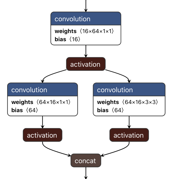
It first has a squeeze layer. This is a 1×1 convolution that reduces the number of channels, for example from 64 to 16 in the above picture. The purpose of the squeeze layer is to compress the data, so that the 3×3 convolution doesn’t need to learn so many parameters.
This is followed by an expand block that has two parallel convolution layers: one with a 1×1 kernel, the other with a 3×3 kernel. These conv layers also increase the number of channels again, from 16 back to 64. Their outputs are concatenated, so the output of this fire module has 128 channels in total.
SqueezeNet has eight of these Fire modules in succession, sometimes with max pooling layers between them. There are no fully-connected layers. At the very end is a convolution layer that performs the classification, followed by global average pooling. (Interestingly, the classification layer both has ReLU and softmax applied to it.)
ImageNet classification accuracy:
| parameters | top-1 | top-5 | |
|---|---|---|---|
| SqueezeNet v1.1 | 1.25 M | 57.5% | 80.3% |
This is similar to the AlexNet score from 2012, but keep in mind that these were no longer state-of-the-art scores in 2016 when the SqueezeNet paper came out.
Speed test (in seconds):
| CPU | GPU | ANE | |
|---|---|---|---|
| iPhone 11 | 0.0079 | 0.0118 | 0.0035 |
| iPhone XS | 0.0105 | 0.0164 | 0.0046 |
| iPhone X | 0.0129 | 0.0205 | n/a |
SqueezeNet is among the fastest architectures, simply because it has relatively few layers and learned parameters. But this speed comes at a cost: SqueezeNet gives worse results than all the other architectures from this blog post. These days, you can get better results with other architectures and a similar number of parameters.
I don’t think a lot of people today use SqueezeNet, but when you train an image classifier with Turi Create, SqueezeNet v1.1 is still one of the options.
Note: The Core ML version of SqueezeNet that is available for download from Apple’s developer site is actually wrong. Its preprocessing layer adds the mean RGB value (123, 117, 104) to the pixels of the input image but it should subtract them instead.
MobileNet v1 (2017)
Paper: MobileNets: Efficient Convolutional Neural Networks for Mobile Vision Applications
Source code and checkpoints: TensorFlow models
I’ve written about MobileNet v1 before. This architecture goes back to 2017, which is a long time ago in the deep learning field, but it’s still a good choice because of its simplicity.
The idea: Replace expensive convolution layers by a cheaper depthwise separable convolution, which is a 3×3 depthwise convolution layer followed by a 1×1 conv layer. This requires a lot fewer learned parameters than a regular convolution but approximately does the same thing.

MobileNet v1 consists of 13 of these blocks in a row. It does not use max pooling to reduce the spatial dimensions, but some of the depthwise layers have stride 2. At the end is a global average pooling layer followed by a fully-connected layer or a 1×1 convolution for doing the classification.
Often ReLU6 is used as the activation function instead of plain old ReLU.
Note: The ReLU6 activation function is not natively supported by Core ML. Instead, you have to use four different layers to accomplish this: first a regular ReLU, then a multiplication by -1, a thresholding operation at -6, and finally multiplication by -1 again.
When I compared the speed of ReLU6 against ReLU, the model with regular ReLU ran significantly faster on the GPU (inference time was ~75% of the ReLU6 model), although there was no noticable difference on the ANE. When fine-tuning MobileNet, it makes sense to replace the ReLU6 layers with regular ReLU for a nice speed boost if you’re targeting older devices. Or replace it with a single custom layer that utilizes MPSCNNNeuronReLUN.
Update 22 Apr: If you don’t mind making your model iOS 13+, you can use a ClipLayer with minimum value 0 and maximum value 6. That does the same thing as ReLU6. However, I recently ran into a bug where a Core ML model with such a clip layer on the GPU set everything to zero; on the CPU and ANE it was fine.
ImageNet classification accuracy:
| parameters | top-1 | top-5 | |
|---|---|---|---|
| MobileNet v1 | 4.24 M | 70.9% | 89.9% |
More than 3 times the parameters of SqueezeNet but also a much better score!
Speed test (in seconds):
| CPU | GPU | ANE | |
|---|---|---|---|
| iPhone 11 | 0.0193 | 0.0243 | 0.0050 |
| iPhone XS | 0.0226 | 0.0362 | 0.0064 |
| iPhone X | 0.0237 | 0.0374 | n/a |
MobileNet has a hyperparameter called the depth multipler (confusingly, also named the “width” multiplier) that lets you choose how many channels are used by the convolution layers. You use this to directly increase or decrease the number of learned parameters. Here, I’ve assumed a depth multiplier of 1.0.
If you use a larger multiplier, the model will give better results but it will also use more parameters and therefore be slower. Conversely, a smaller multiplier makes the model faster but gives worse results.
For example, with multiplier 0.5, MobileNet has 1.34M parameters, which is similar to SqueezeNet. It also runs at roughly the same speed, but has a higher accuracy of 63.3% (top-1).
MobileNet v2 (2018)
Paper: MobileNetV2: Inverted Residuals and Linear Bottlenecks
Source code and checkpoints: TensorFlow models
Core ML model: Download from Apple developer website (this uses depth multiplier 1.4)
I’ve also written about MobileNet v2 before, so check out that blog post for more details.
The idea: Like v1, use depthwise convolutions, but rearrange them like so:

The depthwise convolution is now in the middle. Before the depthwise layer is a 1×1 convolution known as the expansion layer. This increases the number of channels. After the depthwise layer is another 1×1 convolution that reduces the number of channels again, known as the projection layer or the bottleneck layer.
Note: This is exactly the opposite of what SqueezeNet does: it first reduces, then expands.
When the number of channels going into the block is the same as the number of channels coming out (64 in the above picture), there is also a residual connection. Just like in ResNet, this helps to improve the flow of gradients during the backwards pass.
The authors of MobileNet v2 call this an inverted residual because it goes between the bottleneck layers, which have only a small number of channels. Whereas a normal residual connection from ResNet goes between layers that have many channels.
As before, the activation function is ReLU6. However, there is no activation behind the bottleneck layer. Hence the linear bottlenecks from the paper’s title. Since this layer produces low-dimensional data, the authors of the paper found that using a non-linearity after this layer actually destroyed useful information.
The full MobileNet v2 architecture consists of 17 of these building blocks in a row. This is followed by a regular 1×1 convolution, a global average pooling layer, and a classification layer.
ImageNet classification accuracy:
| parameters | top-1 | top-5 | |
|---|---|---|---|
| MobileNet v2 | 3.47 M | 71.8% | 91.0% |
Much fewer parameters than v1 and a slightly improved score on the classification benchmark.
Speed test (in seconds):
| CPU | GPU | ANE | |
|---|---|---|---|
| iPhone 11 | 0.0190 | 0.0185 | 0.0051 |
| iPhone XS | 0.0229 | 0.0284 | 0.0064 |
| iPhone X | 0.0276 | 0.0357 | n/a |
Even though it uses fewer parameters, MobileNet v2 does not run massively faster than v1 and sometimes can even be slower. One explanation is that v2 has more layers, but this also seems to be a Core ML issue. When implemented using Metal Performance Shaders, v2 is definitely a lot faster.
As with v1, you can use the depth multiplier hyperparameter to determine how many channels are used by the model’s convolution layers. For example, with a multiplier of 1.4, the top-1 accuracy improves to 75.0%. With a multiplier of 0.75, the top-1 accuracy drops to 69.8%. (The measurements in table were taken with multiplier 1.0.)
Note: In the picture of the MobileNet v2 layers above, you may have noticed how the 1×1 conv layers have a bias but the depthwise layer has batch norm. That’s just an artifact of this particular TensorFlow graph. The TF model was actually trained with batch norm behind the conv layers. When it was converted to a frozen graph, those batch norm layers were “folded” into the conv layers, but for some reason this wasn’t done for the depthwise layers. At inference time, Core ML should fold away those remaining batch norm layers anyway. Batch norm layers are really only important during training.
MnasNet (2018)
Paper: MnasNet: Platform-Aware Neural Architecture Search for Mobile
Source code and checkpoints: TensorFlow TPU
The idea: Use neural architecture search (NAS) to find an architecture that is specifically suited for mobile devices.
The objective is to find a model that achieves a good trade-off between accuracy and latency. During the search, the latency of the potential new architectures is directly measured by executing them on mobile phones. This is called platform-aware neural architecture search.
Measuring the speed of the model on-device is better than estimating it from the number of FLOPS. But since this is a paper by Google, they primarily used Pixel phones, not iPhones. So their results are not necessarily representative for iOS.
Note: There is also a NASNet without the “m”. This model was also found through architecture search, but it is not specifically intended for use on mobile.
The model they found looks like this:
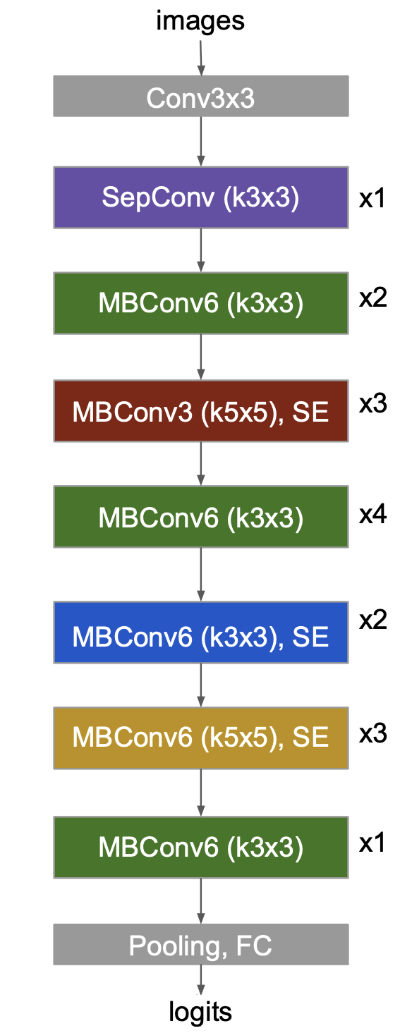
Illustration from the MnasNet paper but flipped upside down.
This is the MnasNet-A1 architecture. It consists of a number of different building blocks that may be repeated multiple times. Some of these use convolution layers with 3×3 kernels, others use 5×5 kernels. This organization may seem arbitrary but that’s what the search found as the best model architecture.
The model starts out with these layers:
- regular 3×3 convolution with 32 filters
- 3×3 depthwise convolution
- 1×1 convolution with 16 filters and linear activation
These are the Conv3x3 and SepConv blocks in the illustration. This is very similar to what MobileNet v2 does.
The next building block is called MBConv6. Again, this is pretty much the same as MobileNet v2:
- 1×1 expansion layer that increases the number of channels by a factor 6
- 3×3 depthwise conv
- 1×1 bottleneck layer that reduces the channels
- residual connection from the previous bottleneck layer (if it has the same number of channels)
The other buildings blocks in MnasNet are variations of the following:
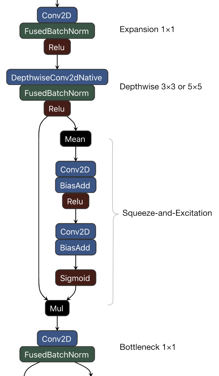
Again, this has an expansion layer, a depthwise convolution, and a bottleneck layer at the end (and possibly a residual connection to the previous bottleneck). In the MBConv3 blocks, the expansion layer uses a factor 3 instead of 6. Sometimes the depthwise convolution is 5×5 instead of 3×3.
The new thing is the addition of a squeeze-and-excitation (SE) module. The idea for this technique comes from the paper Squeeze-and-excitation networks. Note that the SE module was explicitly made part of the architecture search space — it’s not something the search came up with on its own.
Here’s what SE does: First, there is a global average pooling operation (the Mean layer in the illustration above) that reduces the spatial dimensions of the feature map to 1×1. If the feature map had dimensions H×W×C, it is now just a vector with C elements. This is the “squeeze”.
Note: The squeeze in SqueezeNet had another meaning: there it reduced the number of channels, not the spatial dimensions.
Next is the “excitation” part: This is performed by two 1×1 convolution layers with a non-linearity in between (ReLU in this case). The first conv layer massively reduces the number of channels by a factor of 12 or 24, the second conv layer increases the number of channels again to C. A sigmoid is applied to scale the results to be between 0 and 1.
Note: In the original SE-Net paper, they use fully-connected (FC) layers instead of 1×1 convolutions. Since the feature map is only 1×1 pixel in size, these two operations are mathematically equivalent.
What’s the purpose of all this? The idea is that the SE module will learn which features are important. It first compresses the channels vector, then tries to restore it again. The result is that only the most important channels will survive.
The output of the SE branch is combined with the output from the depthwise layer through multiplication (the Mul layer in the illustration). This multiplication works on the channel dimension, and since the output of the sigmoid is between 0 and 1, this simply makes the activation values smaller in channels that are considered to be less important.
As the original paper says, “… the SE block learns how to weight the incoming feature maps.” This helps to increase the accuracy of the model and it’s pretty cheap because the SE layers are small.
The final MnasNet architecture they ended up with is similar in nature to MobileNet v2, except for details such as the sizes of the convolution filters — and obviously the addition of SE. This is not as big a coincidence as it may seem, since the way they chose the architecture search space was heavily influenced by MobileNet to begin with.
Also interesting is that MobileNet v3 (coming up next) starts out from MnasNet-A1, so obviously these model designs have influenced each other.
ImageNet classification accuracy:
| parameters | top-1 | top-25 | |
|---|---|---|---|
| MnasNet-A1 | 3.9 M | 75.2% | 92.5% |
| MnasNet-A3 | 5.2 M | 76.7% | 93.3% |
MnasNet clearly outperforms MobileNet v2, with only 12% or so more parameters, so those architecture changes were effective.
The paper also mentions an A3 variant of MnasNet. This actually scores better than ResNet-50 but is 30% larger and slower than A1.
Speed test (in seconds):
| CPU | GPU | ANE | |
|---|---|---|---|
| iPhone 11 | 0.0180 | 0.0166 | 0.0136 |
| iPhone XS | 0.0219 | 0.0225 | 0.0195 |
| iPhone X | 0.0241 | 0.0318 | n/a |
Speed tests are for MnasNet-A1. On CPU and GPU, MnasNet-A1 is marginally faster than MobileNet v2, but not on the Neural Engine. Core ML only partially uses the ANE to run this model. I suspect this is because of the broadcasted multiply used by the SE module.
Conclusion: This model is a bit better and faster than MobileNet v2, but not if you want to use the Neural Engine. In theory, MobileNet v3 should be an improvement over MnasNet-A1 but in the next section you’ll see that I can’t confirm this.
MobileNet v3 (2019)
Paper: Searching for MobileNetV3
Source code and checkpoints: TensorFlow models
Version 3 is the latest incarnation of MobileNet. The architecture was partially found through automated network architecture search (NAS).
The idea: Use MnasNet-A1 as the starting point but refine it using NetAdapt, an algorithm that automatically simplifies a pre-trained model until it reaches a given latency, while keeping accuracy high. They also made a number of improvements by hand.
Essentially, version 3 of MobileNet is a hand-crafted improvement over MnasNet.
The main changes are:
- expensive layers were redesigned
- use of Swish instead of ReLU6
- squeeze-and-excitation modules (SE)
MobileNet v1 and v2 both begin with a regular 3×3 convolution layer that has 32 filters. It turns out this is a relatively slow layer. It has only a few weights but it does need to work on a large 224×224 feature map. Experimentation showed that 16 filters is sufficient. This doesn’t save a whole lot of parameters but it does give a worthwhile speed-up.
Note: This result doesn’t surprise me, because this blog post shows that 10 of the 32 filters in pretrained MobileNet v1 have very small weights and can therefore be pruned.
Where previous versions of MobileNet used ReLU6 as the activation function, v3 uses a version of Swish called hard swish or h-swish:
h_swish(x) = x * ReLU6(x + 3) / 6
Regular swish does x * sigmoid(x) but because sigmoid is expensive to compute, this is replaced by ReLU6. Clever trick, but only if you can do ReLU6 quickly…
Recall that Core ML does not directly support ReLU6 but requires a four-layer workaround that is itself rather expensive. h-swish adds three more layers to this (one addition and two multiplications). So that’s 7 layers total, yikes.
The MobileNet paper is from Google, so naturally they’re more concerned with performance on Android devices — these design choices are made with Google Pixel hardware in mind. The creators of MobileNet v3 also added an optimized h-swish implementation to TensorFlow Lite, while Core ML obviously does not have such an optimized operator.
Spoiler alert: MobileNet v3 is by no means slow, but it’s also not reaching its full potential on iOS using the standard Core ML layers.
Note: I did not perform this experiment, but perhaps on iOS it’s actually faster to do regular swish using a sigmoid than using the ReLU6 trick… If you’re primarily going to target the CPU or GPU with this model, it might make sense to implement h-swish as a single custom layer (it’s a one-liner in Metal). Keep in mind that custom layers currently don’t work on the ANE; however, that may not be a big issue, as today’s ANE hardware can’t handle MobileNet v3 anyway for other reasons that we’ll get into shortly.
Not all of the model uses h-swish: the first half of the layers use regular ReLU (except after the first conv layer). The MobileNet creators found that h-swish was only beneficial on the deeper layers. And because feature maps tend to be larger in the early layers, calculating their activations is more costly, so they chose to simply use ReLU (not ReLU6) on those layers as it is cheaper than h-swish.
As mentioned, MobileNet v3 uses the same structure as MnasNet-A1. Here is a picture of the main building block:
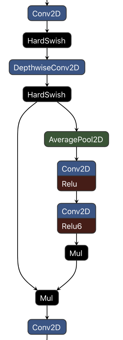
There are a few small differences with MnasNet:
- the activation is h-swish (but as mentioned in the earlier layers it is ReLU)
- the number of filters used by the expansion layers is different (the NetAdapt algorithm was used to find optimal values for these)
- the number of channels that are output by the bottleneck layers may be different (also found by NetAdapt)
- the squeeze-and-excitation (SE) modules only reduce the number of channels by a factor 3 or 4
- instead of a sigmoid, the SE module uses the formula
ReLU6(x + 3) / 6as a rough approximation (just like what h-swish does)
Note: If you’re wondering where that ReLU6(x + 3) / 6 happens, the Mul layer in the right branch multiplies by 0.16667, so that’s the division by 6. The ReLU6 is fused into the conv layer. But where is the x + 3 part? The TFLite converter was clever and actually added 3 to the bias values of the conv layer, a clever micro-optimization that saves doing the addition in a separate layer. We could do this optimization in the Core ML model too and save a layer.
The final optimization involves the layers at the end.
In MobileNet v2, just before the global average pooling layer, is a 1×1 convolution that expands the number of channels from 320 to 1280, so that we have a lot of features that can be used by the classifier layer (or whatever else you stick on top of this backbone). But a big conv layer like that is also relatively slow compared to the rest of the model.
In MobileNet v3, this layer is placed behind the global average pooling layer so that it works on a much smaller feature map (1×1 instead of 7×7) and is therefore much faster. This small change also allows us to remove the previous bottleneck layer and depthwise filtering layer. In total they were able to remove three expensive layers with no loss in accuracy.
Here is an illustration of the model’s output stage:
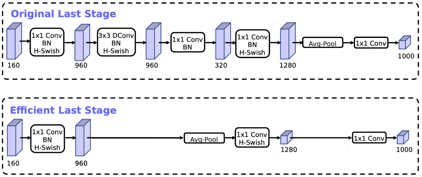
Figure from the paper, slightly modified.
(Note that there is now no batch normalization following these final conv layers.)
Due to these additional improvements, MobileNet v3 is faster than MnasNet with the same accuracy, even though they use the same kind of building block and MobileNet has more parameters!
At least, on Pixel phones… I don’t see these speed improvements on the iPhone. My guess is that it’s primarily due to all these ReLU6 layers, but I haven’t investigated in full detail yet.
By the way, there are several variations of MobileNet v3:
- Large: what I described above
- Small: this has fewer building blocks and smaller numbers of filters
- Large minimalistic: like Large, but doesn’t have SE, h-swish, 5×5 convolutions
- Small minimalistic: likewise for the Small variant
MobileNet v3 also still uses the concept of a depth multiplier. So there are lots of ways you can tweak the size and shape of this model. Like the previous iterations, this architecture doesn’t just define a single model but a whole family of models.
Tip: The Searching for MobileNetV3 paper isn’t just about image classification. It also describes how to use it for object detection (as a drop-in replacement for the backbone in SSDLite) and proposes a new extension for semantic segmentation (LR-ASPP or Lite Reduced Atrous Spatial Pyramid Pooling). Worth checking out if you’re into that sort of thing.
ImageNet classification accuracy:
| parameters | top-1 | top-5 | |
|---|---|---|---|
| MobileNet v3 (small) | 2.9 M | 67.5% | 87.7% |
| MobileNet v3 (large) | 5.4 M | 75.2% | 92.2% |
The accuracy of the Large variant is nearly the same as ResNet-50. It’s a little lower than MnasNet-A3, which has a comparable number of parameters.
It is definitely better than MobileNet v2 with a 1.0 depth multiplier, but that also has fewer parameters (3.47M). I’d say it’s fairer to compare it to v2 with 1.4 depth multiplier (6M parameters), which also has 75% top-1 accuracy.
The Small variant can be compared to v2 with depth multiplier 0.75 (has 2.6M parameters). Interestingly enough, v2 scores better there (top-1 of 69.8%).
Speed test (in seconds):
| CPU | GPU | ANE | ||
|---|---|---|---|---|
| MobileNet v3 (small) | iPhone 11 | 0.0063 | 0.0106 | 0.0102 |
| iPhone XS | 0.0071 | 0.0176 | 0.0164 | |
| iPhone X | 0.0093 | 0.0211 | n/a | |
| MobileNet v3 (large) | iPhone 11 | 0.0152 | 0.0192 | 0.0169 |
| iPhone XS | 0.0174 | 0.0264 | 0.0221 | |
| iPhone X | 0.0219 | 0.0332 | n/a |
The above measurements are for a depth multiplier of 1.0. You can also download checkpoints made with a 0.75 multiplier but I didn’t test those.
Conclusion: The large v3 model outperforms v2 in accuracy and it’s a little faster on CPU and GPU. However, it’s much slower on the Neural Engine — debugging shows that Core ML runs certain parts of this model on the GPU.
Note: Why does the ANE have problems with this model? I don’t know for sure but my guess it’s related to the squeeze-and-excitation blocks. At the end of such a block, we do a broadcasted multiply of a 1×1×C tensor with a H×W×C tensor and I suspect that operation is not available on the Neural Engine (yet?).
Despite the extra hand-tuning of the architecture, MobileNet v3 doesn’t run any faster than MnasNet-A1 on the iPhone. I believe this is primarily an issue with the overhead Core ML introduces in things like ReLU6. This unfortunately undoes the other speed improvements. It may be possible to fix this with custom layers.
I’m not sure I can recommend using this architecture with Core ML at this point: accurracy is better, speed is roughly the same in the best case, way slower in the worst case, and the model takes up 1.5 times more space in the app bundle.
You’ll have to decide for yourself if the better results are really worth it, or if maybe it’s better to stick with a simpler architecture such as MobileNet v2.
BlazeFace (2019)
Paper: BlazeFace: Sub-millisecond Neural Face Detection on Mobile GPUs
Source code and checkpoints: MediaPipe
BlazeFace is a face detection model from Google designed for mobile GPUs. You can use it as part of MediaPipe, which is a C++ framework for building computer vision pipelines. (I also recently ported BlazeFace to PyTorch.)
Even though it wasn’t intended to be general-purpose computer vision model, I’m including BlazeFace in this blog post because of its lightweight feature extractor. According to the paper, this feature extractor was designed specifically for object detection but that doesn’t mean we can’t repurpose it for other tasks. 😁
Interestingly, this paper — even though it’s from Google — specfically mentions the iPhone and Metal Performance Shaders (but not the Neural Engine).
The main building block in this architecture is called the BlazeBlock:
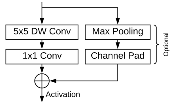
Figure taken from the paper.
In the left branch is a depthwise separable convolution, just like in MobileNet v1. The right branch is a residual connection.
They made the following changes compared to MobileNet:
Increased the kernel size of the depthwise convolutions to 5×5. The rationale for this is that depthwise convolution is relatively cheap compared to the 1×1 convolution, so you might as well make it larger. This is also what happens in MnasNet, though MnasNet doesn’t do it everywhere.
The residual connection is actually between the depthwise layers, not between bottleneck layers (as is done in MobileNet v2).
There is always a residual connection. If the number of channels changes due to the 1×1 convolution, a channel padding layer is added that simply appends empty feature maps to the back of the tensor.
Some of the depthwise layers have stride 2. When that happens, the residual branch also includes max pooling.
The activation function is regular ReLU (not ReLU6).
The BlazeFace feature extractor has 16 of these building blocks in a row. It’s a pretty simple architecture, which is why it is fast.
The input image size for BlazeFace is 128×128, which is smaller than the other models discussed in this blog post (they are typically 224×224 or 227×227). The output features are 8×8×96, which is also smaller than usual.
Note: The paper also mentions a “double” BlazeBlock, which has two sets of convolutions in the left branch. However, the pretrained model from MediaPipe only has single BlazeBlocks.
ImageNet classification accuracy:
| parameters | top-1 | top-5 | |
|---|---|---|---|
| BlazeFace | 0.1 M | ? | ? |
The paper does not mention ImageNet accuracy scores for the feature extractor. However, it does look at average precision (AP) on a face detection dataset. On that task, the full BlazeFace face detection model scores higher than MobileNetV2-SSD.
Of course, that is not evidence that BlazeFace’s feature extractor is better than MobileNet’s, but I also don’t expect it to be much worse for a similar number of learned parameters — which is only 100k for BlazeFace!
But let’s not get carried away: the paper doesn’t explain the configuration of the MobileNet v2 model they used, and the BlazeFace model as described in the paper is not exactly the same as the downloadable one.
So, unless someone retrains BlazeFace on ImageNet, we won’t know how it really stacks up.
Note: If you want to use this feature extractor in your own models, you may need to retrain it on ImageNet for a few epochs, as it is currently trained on faces only.
Speed test (in seconds):
| CPU | GPU | ANE | |
|---|---|---|---|
| iPhone 11 | ? | ? | ? |
| iPhone XS | ? | ? | ? |
| iPhone X | ? | ? | n/a |
The PyTorch → ONNX → Core ML conversion gave errors on the channel padding layer, so I wasn’t able to make a Core ML model to do speed measurements. Since the BlazeFace feature extractor only has 100k parameters and works on smallish 128×128 images, I’m betting it will be plenty fast…
Note: It should be possible to do channel padding using the ConstantPaddingLayer that was introduced with Core ML 3, but I think the ONNX converter puts the padding amounts in the wrong order. I didn’t feel like fixing it because we don’t have ImageNet accuracy scores anyway.
Conclusion: BlazeFace’s feature extractor may be worth experimenting with in your model designs. It’s small and fast, but I don’t have any data on how well it actually performs compared to the other models.
TinyYOLO / Darknet (2016-2018)
Paper: YOLO9000: Better, Faster, Stronger, YOLOv3: An Incremental Improvement
Source code and checkpoints: pjreddie.com/darknet/yolo/
Core ML model: Download from Apple developer website
I’ve written about YOLO a few times before on this blog. YOLO is a fast, one-stage object detector. It also comes in a smaller version that is more suitable for use on mobile, TinyYOLO.
Just like BlazeFace, I’m including TinyYOLO in this blog post because of its feature extractor, also called Darknet.
Why do I care about the TinyYOLO feature extractor? TinyYOLO on the CPU or GPU is definitely a lot slower than the other popular detection model, MobileNet v2 + SSDLite. But on the Neural Engine it actually appears to be faster… What’s up with that?
My hypothesis is that TinyYOLO’s rather “old fashioned” architecture with just convolution and pooling layers is exactly the kind of thing the ANE likes. Models such as MobileNet that use clever tricks such as depthwise separable convolutions run very well on the GPU but may not make optimal use of the ANE. (Maybe.)
Is this actually true? We’ll see…
Sidebar: It’s unfortunate that Apple doesn’t provide any information whatsoever about how the Neural Engine works and how to take advantage of it. It would be helpful to have a document that says which layer types to avoid, how to design your models to get the most out of the ANE, and so on. It would take away the need for this kind of guesswork.
TinyYOLO v2 is a very simple convnet consisting of eight 3×3 convolutions with max pooling layers in between, and a final convolution layer for doing the bounding box predictions. Feature extraction gives a nice big (13, 13, 1024) tensor.
Since I last wrote about YOLO, version 3 has come out. The first layers in v3 are the same as before:
Layer          kernel   filters
-------------------------------
Convolution    3×3      16
MaxPooling     2×2
Convolution    3×3      32
MaxPooling     2×2
Convolution    3×3      64
MaxPooling     2×2
Convolution    3×3      128
MaxPooling     2×2
Convolution    3×3      256
All convolution layers are followed by batch norm and Leaky ReLU with 0.1 slope.
At this point, the model splits into two branches. The first branch looks like this:
Layer          kernel   filters
-------------------------------
MaxPooling     2×2
Convolution    3×3      512
MaxPooling     2×2
Convolution    3×3      1024
Convolution    1×1      256
-------------------------------
The output of this goes into another 1×1 convolution with 128 filters, which is then upsampled by a factor of 2 and concatenated with the second branch. This is followed by another set of convolutions that do the bounding box predictions, but we’re not interested in that here.
Just like v2, it’s still mostly convolutions followed by max pooling. Nothing fancy.
Note: I’m not entirely sure where the feature extractor ends and where the object detector begins. You probably wouldn’t keep the second branch, as it is mostly there to help detect objects in the higher-resolution feature maps.
The YOLO papers don’t actually explain these tiny variants of the model. Instead, they describe Darknet-19 and Darknet-53, the full-size versions of the feature extractor, which are more complex and also use things like residual connections.
ImageNet classification accuracy:
| parameters | top-1 | top-5 | |
|---|---|---|---|
| TinyYOLO v3 | 8.6 M | ? | ? |
| TinyYOLO v2 | 15 M | ? | ? |
The paper does not give ImageNet scores for the tiny versions, but top-1 score for Darknet-19 is 74.1%, and Darknet-53 is 77.2%. It’s likely that TinyYOLO scores much worse.
Note that v2 has a big convolution at the end with 1024 input and output channels, which is why it has almost double the parameters of v3.
Speed test (in seconds):
| CPU | GPU | ANE | ||
|---|---|---|---|---|
| TinyYOLO v3 | iPhone 11 | 0.0141 | 0.0219 | 0.0054 |
| iPhone XS | 0.0321 | 0.0317 | 0.0079 | |
| iPhone X | 0.0268 | 0.0302 | n/a | |
| TinyYOLO v2 | iPhone 11 | 0.0197 | 0.0230 | 0.0063 |
| iPhone XS | 0.0526 | 0.0318 | 0.0076 | |
| iPhone X | 0.0741 | 0.0290 | n/a |
These measurements were done with the bounding box prediction layers removed.
The input image used with YOLO is 416×416, which is larger than for most other models discussed here. However, I ran the speed tests with 256×256 images to make the comparison fairer (that’s also what the feature extractors were originally trained with). On 416×416 images the models are roughly twice as slow as what’s shown in the table.
Conclusion: Well, I guess my hypothesis was… incorrect! 😅
When looking at just the feature extractors, MobileNet v2 is definitely faster on the GPU — but it’s also faster on the ANE!
So, why does the TinyYOLO object detector run faster than MobileNetV2+SSDLite on the ANE? It must be because of the SSD layers. Without those layers, MobileNet definitely beats YOLO.
Note: To be fair, when I compared TinyYOLO to MobileNet+SSD, the SSD bounding box decoding logic was part of the Core ML model. But with TinyYOLO the decoding was done on the CPU with the Accelerate framework. I don’t know how much this difference affects the speed, but it could be a lot. Maybe I’ll write a future blog post where I compare the performance of object detection models, so I can go into this in more detail.
If you’re building a real-time object detector that needs to run on the Neural Engine, TinyYOLO is probably the better choice (don’t take my word for it: do the measurements yourself). But as a feature extractor, I’d still prefer MobileNet.
Since we also don’t have any ImageNet accuracy figures for TinyYOLO’s feature extractor, I don’t think I can recommend it for that purpose.
Note: What about the full YOLO v3? Personally, I wouldn’t use this on mobile. It’s a pretty big model. It gives more accurate results than MobileNet+SSD but it’s also a lot slower. For speed, you definitely want the tiny version.
SqueezeNext (2018)
Paper: SqueezeNext: Hardware-Aware Neural Network Design
Source code and checkpoints: github.com/amirgholami/SqueezeNext
As the name implies, SqueezeNext is based on SqueezeNet but with a number of architectural improvements.
The new SqueezeNext block looks like this:
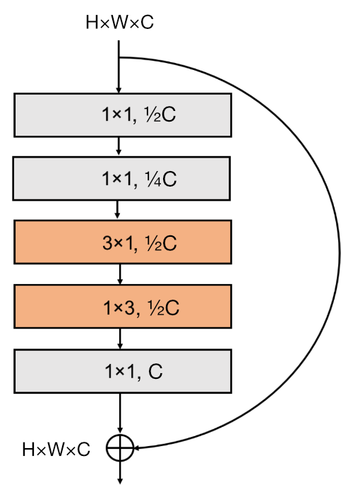
Figure based on the paper.
There are five conv layers in each block, all with batchnorm and ReLU:
The first two layers are bottleneck layers, i.e. 1×1 convolutions that reduce the number of channels. If
Cis the number of input channels, the first bottleneck layer reduces this toC/2, the second one toC/4.As with the original SqueezeNet, these bottlenecks are used to cut back the number of parameters needed by the convolution layers that do the actual filtering. Why use two bottleneck layers in a row? Not sure, but perhaps this gives better results than going from
CtoC/4in a single step. More layers is better!Unlike the original SqueezeNet, there is no longer a 3×3 convolution. Instead, this has been split up into two smaller convolutions: 3×1 and 1×3. These both have
C/2filters. Splitting it into two smaller layers decreases the number of parameters needed. At the same time it increases the depth of the network, which generally improves the model. (Even more layers!)The order of these two convolutions alternates. If this block has 3×1 followed by 1×3, the next block does 1×3 first and 3×1 second, and so on. I guess they do this to keep things interesting.
The fifth and final layer is an expansion layer, a 1×1 convolution that brings the number of channels back to
C.
As is common with modern architectures, there is also a residual connection.
Recall that the original SqueezeNet had convolutions in both branches, but that doesn’t happen here: the residual branch has no convolution in it. However, there is a small exception to this rule…
The blocks in SqueezeNext are organized into four sections. In each new section, the spatial dimensions of the feature maps are halved. To achieve this, the very first bottleneck convolution has stride 2. Now the residual branch for that block must also have a stride 2 convolution, otherwise the outputs of both branches cannot be summed up.
(Also, in this first block, the number of output channels can be different than the number of input channels, so the branch with the residual connection must match that too.)
Note: Curiously, the official Caffe models apply ReLU before the summation of the residual connection with the main branch, but also after. I haven’t seen that in other ResNet-like models before — it seems like a ReLU too many. Contrast this with MobileNet v2, where there is no activation at all at this point.
The very first layer in SqueezeNext is a 7×7 convolution with 64 filters and stride 2. This layer does not use zero-padding. It is immediately followed by max pooling, so the input size of 227×227 pixels is very quickly reduced to 55×55 pixels.
(Unimportant detail: Because of the pooling layer, the first convolution in the very first section has a stride of 1 instead of 2. Not sure why they use a max pooling layer there and not anywhere else.)
At the end of the model is a single fully-connected layer that performs the actual classification. Right before this layer is a bottleneck layer that reduces the number of channels, which saves a lot of parameters in the FC layer, and a global average pooling to reduce the spatial dimensions. (SqueezeNet actually used a conv layer to do the classification, and did global pooling last.)
SqueezeNext, like MobileNet, is not just a single fixed design but a family of possible architectures:
A width multiplier determines the number of filters in each block. The paper examines width multipliers of 1.0, 1.5, and 2.0.
You can also change the number of building blocks used. The paper shows models with 23, 34, and 44 blocks. As you might expect, more blocks gives better results.
You can vary how many blocks there are in each section. For example, the “v5” variant has relatively few blocks in the first two sections (which work on feature maps of sizes 55×55 and 28×28), many blocks in the third section (feature map size 14×14), and only one block in the last section (size 7×7).
In other variants of SqueezeNext, the first bottleneck and the 1×3 and 3×1 layers use group convolution with a group size of two, which cuts the number of parameters in half for those layers. (This is a little bit like making them depthwise convolutions, which is a grouped convolution where the number of groups equals the number of channels.)
The authors of SqueezeNext did not use depthwise separable convolutions on purpose, because these “do not give good performance on some embedded systems due to its low arithmetic intensity (ratio of compute to bandwidth).”
Interesting, because depthwise separable convolutions actually work very well on the iPhone GPU (see the success of MobileNet); the paper does not go into details about what sort of embedded systems they intended SqueezeNext for.
To try out different design approaches, the authors simulated the performance of possible architectures on a hypothetical neural network accelerator chip. This is different from MnasNet, which tries out the architectures on actual hardware. Because of this, I’m not sure how well SqueezeNext’s design decisions translate to the real world — or at least to iPhone hardware.
The paper also shows results for models that use Iterative Deep Aggregation (IDA). Instead of just having a linear sequence of blocks that only does the classification at the very end, with IDA we already make a prediction after each block, and these predictions are then combined with those of the final classification layer. This idea improves accuracy (a little) but at the cost of more parameters. (It doesn’t appear to be a major feature of SqueezeNext.)
ImageNet classification accuracy:
| parameters | top-1 | top-5 | |
|---|---|---|---|
| 1.0-SqNxt-23 | 0.7 M | 59.05% | 82.60% |
| 1.0-SqNxt-44 | 1.2 M | 62.64% | 85.15% |
| 1.0-SqNxt-44-IDA | 1.5 M | 63.75% | 85.97% |
| 2.0-SqNxt-23v5 | 3.2 M | 67.44% | 88.20% |
These are the accuracy scores for a few different variations of the architecture.
The 1.0-SqNxt-44 model can be compared to the old SqueezeNet. While it scores better than the original, its accuracy is still lower than MobileNet v1, even if we compare it with a version of MobileNet that has a similar number of parameters (0.5 depth multiplier, top-1 score 63.3%).
The SqueezeNext paper claims better top-5 accuracy than MobileNet v1 with 1.3× fewer parameters. To get this result, they compare their 2.0-SqNext23v5 model with MobileNet-1.0-224. However… the version of MobileNet they’re using is not as good as the official one — they trained it using the same hyperparameters as their own models, for getting a fairer comparison.
I guess this makes sense but it also makes the claim “better than MobileNet” a bit dubious (especially since the top-1 accuracy of SqueezeNext isn’t actually better).
Speed test (in seconds):
| CPU | GPU | ANE | |
|---|---|---|---|
| iPhone 11 | 0.0203 | 0.0292 | 0.0062 |
| iPhone XS | 0.0307 | 0.0435 | 0.0076 |
| iPhone X | 0.0316 | 0.0537 | n/a |
Measurements are for the largest model, 2.0-SqNxt-23v5. This model has similar accuracy as MobileNet v3 (small) but the speed is waaay worse. (Except on ANE, where MobileNet v3 isn’t doing so well.)
Conclusion: It seems like most of these newer architectures do similar things with bottleneck layers, expansion layers, and residual connections — and SqueezeNext is no exception. I like the idea of splitting up the 3×3 convolution into 3×1 and 1×3, but I’m not sure if it actually works better than depthwise separable convolutions in practice.
SqueezeNext is pretty good for a model with relatively few parameters, but on the iPhone I’d still pick MobileNet over it.
ShuffleNet (2017, 2018)
Paper (v1): ShuffleNet: An Extremely Efficient Convolutional Neural Network for Mobile Devices
Paper (v2): ShuffleNet V2: Practical Guidelines for Efficient CNN Architecture Design
Source code and checkpoints: github.com/megvii-model/ShuffleNet-Series
ShuffleNet is already from a few years ago and it’s been on my to-do list for ages, so I’m using this blog post to finally take a look at it. 😅 There are a few different versions, so let’s start with v1.
The idea: Many of the modern architectures use lots of dense 1×1 convolutions, also known as pointwise convolutions, but they can be relatively expensive. To bring down this cost, we can use group convolutions on those layers. But those have side effects, with can be mitigated using a channel shuffle operation.
A group-wise convolution divides the input feature maps into two or more groups in the channel dimension, and performs convolution separately on each group. It is the same as slicing the input into several feature maps of smaller depth, and then running a different convolution on each.
With two groups, you only need half the parameters because each convolution filter now works on half the input channels and produces half the output channels. (The weights are not shared between the groups — each group still learns its own parameters!)
Note: Group convolution is similar to depthwise convolution. In fact, depthwise convolution is sometimes implemented using the more general grouped convolution. The difference is that with depthwise convolution, each input channel is its own group and there is one output channel for each input channel. With the more general form of group convolution, the number of output channels for each group does not have to equal the number of input channels in the group.
A side effect of grouped convolution is that each output is only derived from a fraction of the inputs, i.e. the output channels are also divided into the same number of groups. This is not ideal because there is no information flow between different groups, which limits the network’s ability to learn interesting things.
The solution is simple: just shuffle things around a bit afterwards.
After the grouped convolution, the channel shuffle operation rearranges the output feature map along the channels dimension, like so:
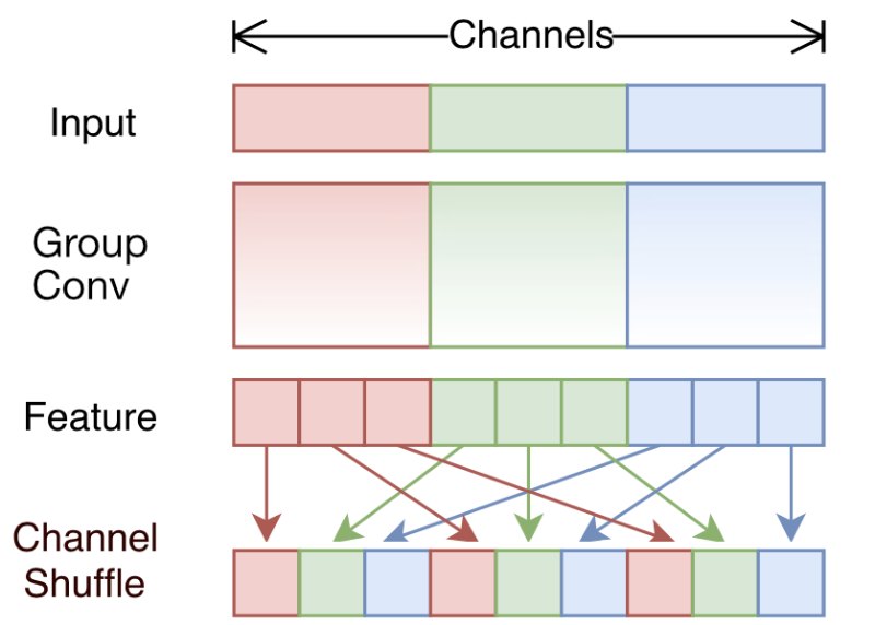
Based on the figure from the paper.
This may look complicated but it can easily be accomplished using basic reshape and transpose operations. If G is the number of groups and K is the number of channels per group, then:
reshape the input tensor from
(N, C, H, W)to(N, K, G, H, W)transpose the
GandKdimensions in the array, so now the tensor has shape(N, G, K, H, W)reshape the tensor back to
(N, C, H, W)
The building block in ShuffleNet v1 is then as follows:
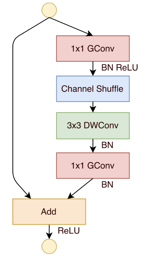
Figure taken from the paper.
The first convolution is a 1×1 bottleneck layer that reduces the number of channels by a factor of 4. This layer uses grouped convolution and is followed by channel shuffle.
The 3×3 layer is a depthwise convolution with batchnorm but without ReLU. Not using ReLU gave better results here.
The final layer is another 1×1 grouped convolution, which is used to expand the number of channels again (to match those of the residual connection). On this layer there is no channel shuffle as the authors found it didn’t make any difference in that spot.
As usual, there is a residual connection.
Sometimes the depthwise layer will have stride 2. In that case, the left branch has a 3×3 average pooling layer inside it and the results are concatenated with the main branch, not added.
The paper discusses experiments on different group sizes, but overall 8 groups seems to give the best results. The more groups, the fewer parameters the model needs and the smaller its computational complexity. Or looking at it differently, for the same amount of complexity you can now have more feature maps and get a better accuracy.
The full architecture starts with a regular 3×3 convolution with stride 2, which is followed by max pooling. Then there are three stages, each with 4 or 8 ShuffleNet blocks. The first block in a stage has stride 2. Finally, there is global average pooling and a fully-connected layer that does the classification.
OK, that’s the architecture of v1. The paper makes a big deal out of these group-wise convolutions, but a little while later the authors changed their minds…
Let’s see what’s up with that and study version 2.
The ShuffleNetV2 paper has an interesting discussion about how different types of layers perform on actual hardware. The authors use those insights to come up with an improved network structure.
When analyzing the speed of the model they realized it’s not really worth doing grouped convolutions after all. These do have the benefit of requiring fewer parameters and computation — but if you then use this to justify having more channels in order to boost the accuracy of the model, the number of memory accesses also goes up. And when it comes to speed, it’s those extra reads and writes that slow the model down.
The new ShuffleNet v2 building block looks like this:
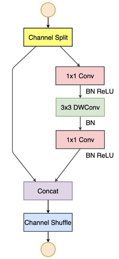
Figure taken from the paper.
Here’s what changed:
- To replace the group convolutions, there is a new channel split operation, which sends half the channels through the left branch and the other half through the right branch — this is like using two groups.
- The 1×1 convolutions are no longer groupwise.
- The convolutions now always have the same number of input and output channels. They found that, when the number of channels stays the same, the amount of memory accesses in the convolution is optimal.
- The shortcut connection is now always concatenated, not summed — this is the reverse operation of the channel split at the beginning. (So, technically speaking it’s no longer a residual connection.)
- The channel shuffle is still there but has moved to the end.
The main reason they’re using concat instead of add on the two branches is that elementwise operations such as addition are relatively expensive — they perform a lot of memory accesses but do little computation. Since it’s possible to merge concat, channel shuffle, and channel split into a single element-wise operation, you can optimize this away.
Note: When the depthwise convolution has stride 2, the left branch is a little different. This gets its own 3×3 depthwise convolution with stride 2, followed by a 1×1 convolution, to make sure the outputs of both branches have the same spatial dimensions (or they cannot be concatenated). There is no channel split operation in such a block, so both branches work on the same data and the concat effectively doubles the number of channels.
Other than the change to the building blocks, the overall structure of the model is the same as in v1, except there is now a big 1×1 convolution layer before the global average pooling and fully-connected layer at the end.
There is also a newer variant, ShuffleNet v2+, which adds hard-swish, hard-sigmoid, and squeeze-and-excite, just like in MobileNet v3.
ImageNet classification accuracy:
| parameters | top-1 | top-5 | |
|---|---|---|---|
| ShuffleNet v1 1.0× (8 groups) | 2.4 M | 68.0% | 86.4% |
| ShuffleNet v2 1.0× | 2.3 M | 69.4% | 88.9% |
| ShuffleNet v2 1.5× | 3.5 M | 72.6% | 90.6% |
| ShuffleNet v2+ (medium) | 5.6 M | 75.7% | 92.6% |
| ShuffleNet v2+ (large) | 6.7 M | 77.1% | 93.3% |
ShuffleNet v1 is on-par with Mobilenet v1 (0.75 depth multiplier).
ShuffleNet v2 with 1.0 scale factor is a bit better than ShuffleNet v1. (The scale factor is like the depth multiplier used in other models. It increases or decreases the number of filters used by the convolution layers throughout the network.)
ShuffleNet v2 with 1.5 scale factor is comparable with MobileNet v2, even slightly better.
ShuffleNet v2+ (medium) is a little better than MobileNet v3 (large) at roughly the same number of parameters.
ShuffleNet v2+ (large) is the best scoring model so far in this blog post, but it’s also the largest.
Speed test (in seconds):
| CPU | GPU | ANE | |
|---|---|---|---|
| iPhone 11 | 0.0139 | 0.0340 | 0.0126 |
| iPhone XS | 0.0156 | 0.0674 | 0.0138 |
| iPhone X | - | - | n/a |
Measurements are for ShuffleNet v2 1.5×. I have no results for iPhone X, as mine runs iOS 12 and this model needs iOS 13 or better due to how the channel shuffle layers were converted (in theory it should be possible to make an iOS 12 version).
Conclusion: The accuracy scores are among the best we’ve seen so far in this blog post. They’re generally better than MobileNet at the same number of parameters.
But… this model does not run well on the GPU at all! I think this is because of the way channel shuffle was converted to Core ML. It ends up being a combination of reshape / transpose / slice / squeeze layers that could be replaced by a single Metal kernel (or at least by a more efficient choice of Core ML layers).
CondenseNet (2017)
Paper: CondenseNet: An Efficient DenseNet using Learned Group Convolutions
Source code and checkpoints: github.com/ShichenLiu/CondenseNet
The idea: Like ShuffleNet v1, use group convolutions for 1×1 layers, but learn the groupings.
The starting point is an architecture similar to DenseNet, where each layer’s output is concatenated with the outputs of all the layers before it. Reusing the features in this way helps to boost accuracy.
However, this kind of dense connectivity may be more than we need, as features from early layers may not always be needed in later layers. The problem, of course, is that you don’t know beforehand which features should be reused.
This is where CondenseNet comes in: during training it learns which features from earlier layers are important enough to keep.
It does this by splitting up the filters from a convolution layer into groups, typically 4 or 8 groups per layer.
Over time, input features that are considered less important are pruned from the model. This is done per group, so a given input feature can be removed from one group of filters but still be used by another group.
When training is done, each group in this layer only keeps 1/C of the original filters where C is known as the condensation factor. C is typically 4 or 8.
At inference time, we don’t have to worry about any of this. However, we do need to ignore feature maps coming from earlier layers that have been pruned away. We also need to rearrange the remaining input channels to assign them to the correct groups. This is done by an index layer, which is just a lookup table.
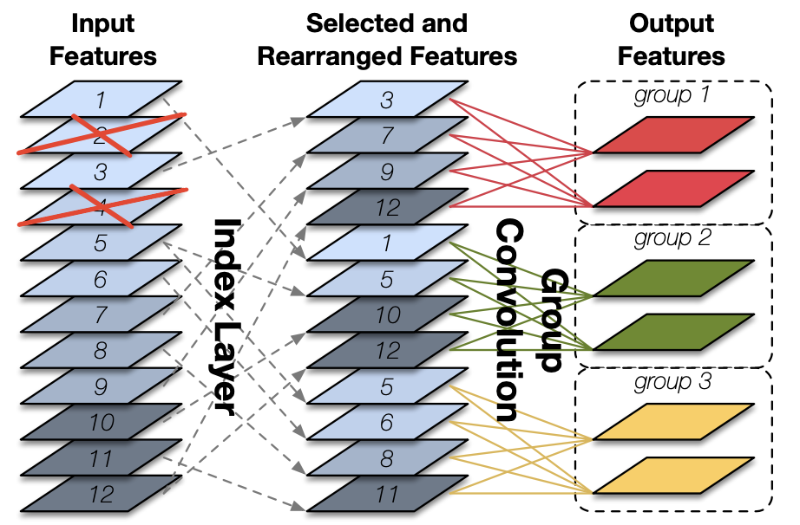
Figure taken from the paper.
The actual convolution can then be done by a normal group convolution, which is a lot more efficient than using a sparse convolution.
This is followed by a channel shuffle operation, just like in ShuffleNet, to improve the information flow between the groups.
ImageNet classification accuracy:
| parameters | top-1 | top-5 | |
|---|---|---|---|
| CondenseNet-74 (8 groups) | 2.9 M | 71.0% | 90.0% |
| CondenseNet-74 (4 groups) | 4.8 M | 73.8% | 91.7% |
These scores are not too bad, comparable to MobileNet and ShuffleNet v1 & v2.
Speed test (in seconds):
| CPU | GPU | ANE | |
|---|---|---|---|
| iPhone 11 | 0.0397 | 0.1642 | 0.0402 |
| iPhone XS | 0.0531 | 0.3586 | 0.0533 |
| iPhone X | - | - | n/a |
Measurements are for the larger model. It looks like the iPhone has a few problems with CondenseNet, especially on the GPU where it is super slow.
(I have no results for iPhone X, as mine runs iOS 12. This model needs iOS 13 or better because the “index layer” is made with a Gather operation.)
Conclusion: Interesting idea, especially since DenseNet-like architectures usually aren’t used on mobile. But as ShuffleNet v2 shows, grouped convolutions weren’t really the answer…
The paper claims that CondenseNet achieves similar accuracy as MobileNet at only half the compute, but compute isn’t the whole story. As the speed test shows, Core ML sort of chokes on this model.
ESPNet (2018)
Paper (v1): ESPNet: Efficient Spatial Pyramid of Dilated Convolutions for Semantic Segmentation
Paper (v2): ESPNetv2: A Light-weight, Power Efficient, and General Purpose Convolutional Neural Network
Source code and checkpoints: github.com/sacmehta/EdgeNets
Core ML model: iOS demo app
I’m mostly interested in ESPNet v2 but let’s first look at the ideas from v1.
The idea: Decompose the standard convolution layer into pointwise convolutions, followed by a spatial pyramid of dilated convolutions.
Splitting up convolution into a 1×1 layer plus “something else” is quite common, but here the something else is different from what we’ve seen so far.
The Efficient Spatial Pyramid (ESP) module looks likes this:
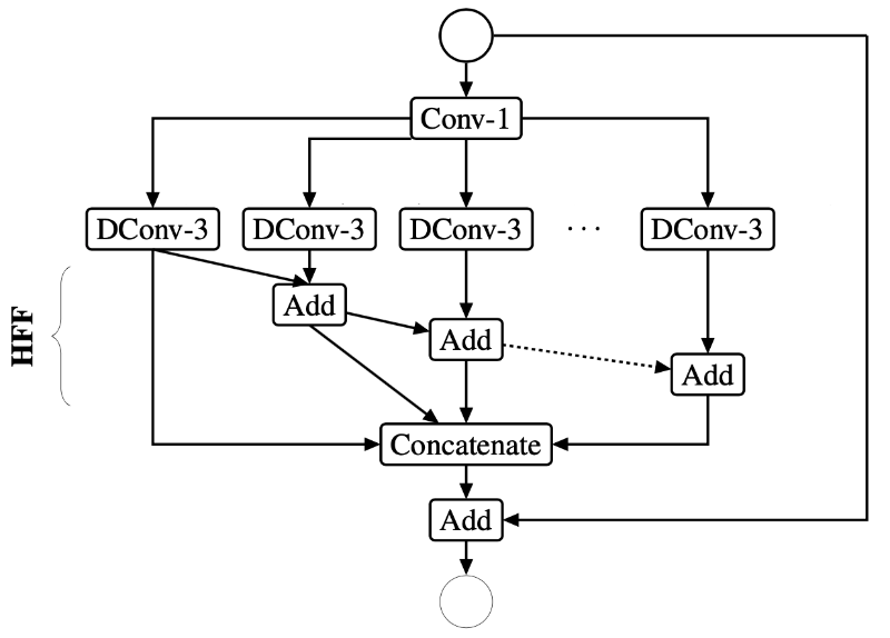
Figure taken from the paper.
As is usual, the 1×1 convolution (Conv-1 in the picture) is a bottleneck layer that reduces the number of channels. There is a “width divider” hyperparameter, K, that determines by how much. If N was the original number of output channels, then the bottleneck layer has N/K output channels.
The spatial pyramid is made up of several parallel 3×3 conv layers (DConv-3). These are dilated convolutions with a dilation rate of 1, 2, 4, 8, 16, and so on. Making the convolutions dilated enlarges the receptive field that can be learned from. There are K of these dilated kernels and each one has N/K filters.
Afterwards, the output from the spatial pyramid is concatenated along the channel dimension, so the final number of output channels is N again.
Note: The Add layers perform hierarchical feature fusion (HFF). This is done to remove artifacts such as checkerboard patterns that occur due to the gaps in the dilated convolutions.
Of course there is also the inevitable residual connection to help with gradient flow.
It may seem like the ESP module does a lot more work than a standard convolution but it actually has fewer parameters (thanks to the pointwise layer) and has a much larger receptive field (thanks to the dilated convolutions).
ESPNet v1 was designed specifically for semantic segmentation. ESPNet v2 builds on the ideas of v1 and is intended for general-purpose computer vision tasks and even things like language modeling.
The idea: Make the dilated convolutions depthwise separable.
The new building block is named EESP, which stands for Extremely Efficient Spatial Pyramid, and looks like this:

Based on the figure from the paper.
Just like in ShuffleNet, this uses group convolution for the 1×1 bottleneck layer (the first GConv-1 in the picture), although it doesn’t do channel shuffle.
The dilated convolution is now split into two parts: first a 3×3 depthwise layer that is also dilated (DDConv-3), followed by a 1×1 pointwise layer.
Rather than computing K separate 1×1 layers, they concatenate the results from the dilated layers and then apply a single 1×1 grouped convolution to that (GConv-1 at the bottom). This is equivalent but more efficient.
The activation function is PReLU.
The full architecture begins with a regular conv layer with stride 2. This is followed by three stages. Each stage starts with a strided EESP block to halve the spatial dimensions and double the number of channels. The rest of the stage is made up of several regular EESP blocks. After these three stages, there are a couple more convolution layers, global average pooling, and a fully-connected classifier layer.
The strided EESP has stride 2 on the dilated convolutions. The residual connection is replaced by average pooling and concatenation, which serves to double the number of channels. (This is faster than doubling the number of filters in the conv layers.)
In addition, they add another, long-range, shortcut connection that goes all the way back to the input image. This new connection has one or more average pooling layers, followed by a depthwise separable convolution. The idea is that this long-range connection pulls in some extra spatial information that might otherwise be lost by the downsampling.
ImageNet classification accuracy:
| parameters | top-1 | top-5 | |
|---|---|---|---|
| ESPNet v2 2.0× | 3.49 M | 72.1% | 90.4% |
| ESPNet v2 | 5.9 M | 74.9% | ? |
This is similar to the scores of MobileNet v2 and ShuffleNet v2. The paper mentions that the number of FLOPS is less for ESPNet v2, but as we all know, FLOPS don’t tell the full story when it comes to speed.
Note: As is common with these modern model types, ESPNet also employs a width scaling factor. I’m not sure what scaling factor the 5.9M-parameter model uses; the paper doesn’t mention this. There is also no pretrained model for this size available.
Speed test (in seconds):
| CPU | GPU | ANE | |
|---|---|---|---|
| iPhone 11 | 0.0517 | 0.0231 | ? |
| iPhone XS | 0.0620 | 0.0341 | ? |
| iPhone X | 0.0627 | 0.0409 | n/a |
Measurements are for ESPNet v2 with 2.0× scale factor.
Note: I was unable to get results on the ANE because Core ML failed with a “Program Inference overflow” error. I’ve seen that a few times on untrained models (which have random weights) but this one was actually trained. Weird.
Conclusion: It’s rather slow. I think one issue is that splitting up a convolution into many smaller layers isn’t necessarily beneficial. The overhead of performing many small operations may undo any potential speed gains.
The extra complexity of this model isn’t worth the small increase in accuracy. By just counting the number of FLOPS the model might be “faster” in theory, but in practice it’s slower because the model structure is not hardware friendly.
DiCENet (2019)
Paper: DiCENet: Dimension-wise Convolutions for Efficient Networks
Source code and checkpoints: github.com/sacmehta/EdgeNets
This is from the same people as ESPNet. By the way, the company some of these authors were affiliated with, Xnor.ai, was recently purchased by Apple for 💰💰💰. Who knows if we’ll see some of this tech in iOS at some point.
The idea: Replace regular convolution with dimension-wise convolution and fusion.
Say what now? Most of the neural networks discussed in this blog post are built around some clever new idea to split up plain old convolution into smaller and more efficient operations. This one is no exception — we just have to figure out what “dimension-wise” means.
As you know, with depthwise convolution and group convolution we slice the input tensor along the channel dimension, and each convolution filter runs on its own subset of the channels. But why not slice along the width or height dimensions too?
The drawback of a depthwise convolution is that it needs to be followed by a 1×1 layer to mix up the channels. As the DiCENet paper points out, all these pointwise convolutions account for 90% of all operations in models such as MobileNet. ShuffleNet attempted to fix this by making the 1×1 convolutions faster using grouped convolution, but we can maybe do better.
With a dimension-wise convolution — or “DimConv” — the convolution happens across each dimension of the input data.
If the tensor is D×H×W, we can perform convolution along three possible axes:
H×W— this is the well-known depth-wise convolution. The input tensor is sliced along the channel axis, and the filter window slides across the spatial dimensions (i.e. across the image’s width and height).D×H— this is a width-wise convolution. Now the input tensor is sliced along theWaxis, and the filter window slides across an image of sizeD×H.D×W— this is a height-wise convolution. The input tensor is sliced along theHaxis and the filter window works on an image of sizeD×W.
Note: In this blog post I usually use C to refer to the number of channels, but the paper uses D (for depth), so I’m doing that here too.
We want these convolutions to be lightweight. With depth-wise convolution, there is one filter for every channel. We do the same thing for the other two types:
- width-wise convolution has one filter for every x-position
- height-wise convolution has one filter for every y-position
This means there are D depth-wise filters, W width-wise filters, and H height-wise filters, so in total there are D×H×W filters in the DimConv layer (usually of size 3×3).
Finally, the outputs from the depth-wise, width-wise, and height-wise convolutions are concatenated along the channel dimension (in an interleaved manner).
Note: The size of the output feature map of a depth-wise convolution is the same as its input, assuming we’re using zero-padding around the edges. The same is true for width-wise and height-wise convolutions. If the input is D×H×W, then the output of each of these three types of kernels is also D×H×W, and the concatenated output tensor is 3D×H×W.
One small detail: The width-wise and height-wise convolutions depend on the input tensor to have a certain width or height. If you want the DimConv layer to accept arbitrarily sized input images, there should be an upsampling (or downsampling) layer before the width-wise and height-wise convolutions, and a corresponding downsampling (or upsampling) layer afterwards.
Here’s a picture of the main building block, the so-called DiCE unit (which stands for Dimension-wise Convolutions for Efficient networks):
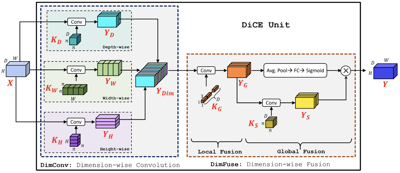
Figure taken from the paper.
On the left is the DimConv layer we’ve just described. On the right is a so-called dimension-wise fusion or “DimFuse” layer that combines the results of DimConv in some interesting fashion.
The DimFuse layer replaces the 1×1 layer that typically follows a depthwise layer. Even though DimConv has encoded information along the three different axes, it has done so independently, and we still need to mix everything up (similar to why ShuffleNet needs channel shuffle).
DimFuse does this in two steps:
Local fusion. The results from DimConv ’s three convolution types are placed interleaved in
Y_Dim, so this tensor containsDgroups of 3 slices of sizeH×W. The “local fusion” stage of DimFuse applies a grouped 1×1 convolution that will combine each group of 3 slices into a single slice. This results inY_G, a tensor of sizeD×H×W.Global fusion. This has two branches:
i. The bottom branch looks at things spatially: it performs a regular depthwise convolution to independently filter each of the
Dchannels inY_G.ii. The top branch looks at the channels: it determines how important each channel is using squeeze-and-excitation. You’ve seen this before: there is an average pooling layer to squash the tensor’s width and height into a single pixel, followed by a fully-connected layer and a sigmoid. In other words, this computes a weighting factor for each channel of
Y_G(and thusY_S).
The paper describes DiCENet, which is really just ShuffleNet v2 but with DiCE units. The building blocks now looks like this:
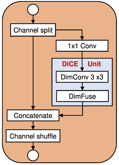
Figure taken from the paper.
In fact, you can take any existing architecture and swap out the blocks for DiCE units and it will work better (or so they say).
ImageNet classification accuracy:
| parameters | top-1 | top-5 | |
|---|---|---|---|
| DiCENet 1.0 | 1.81 M | 66.5% | 86.6% |
| DiCENet 1.5 | 2.65 M | 69.5% | 88.8% |
| DiCENet 2.0 | 3.98 M | 71.0% | 89.8% |
Pretty good scores but not massively better than anything we’ve seen before.
With the 1.0 scale factor it outperforms MobileNet v2 and ShuffleNet v2 at a similar number of parameters.
Speed test (in seconds):
| CPU | GPU | ANE | |
|---|---|---|---|
| iPhone 11 | ? | ? | ? |
| iPhone XS | ? | ? | ? |
| iPhone X | ? | ? | n/a |
I did not try this model because Core ML does not support doing convolutions along the other axes. (Also, I was unable to export the PyTorch model.)
It should be possible to make this work by permuting the tensor, doing a regular convolution, and then permuting back again — but that seems like a hassle. (In fact, this is what the original PyTorch code does.)
Conclusion: Width-wise and height-wise convolutions are an obvious idea once you have depth-wise convolutions, but I certainly wasn’t smart enough to think of them, haha. 😆
Cool idea, but for our purposes it does not seem worth doing as it requires Core ML hacks to get this working. But hey, since Apple now owns Xnor.ai, perhaps we’ll get convolutions along arbitrary axes in Core ML 4…
FBNet & ChamNet (2018)
Paper 1: FBNet: Hardware-Aware Efficient ConvNet Design via Differentiable Neural Architecture Search
Paper 2: ChamNet: Towards Efficient Network Design through Platform-Aware Model Adaptation
Source code and checkpoints: github.com/facebookresearch/mobile-vision
The idea: A more efficient way to perform neural architecture search (NAS) so that it is not necessary to train and evaluate each potential architecture separately.
My blog post isn’t really about NAS so I won’t go into too many details (also, I’m a noob when it comes to NAS). But obviously, a faster way to do architecture search allows you to explore a larger part of the — huge! — design space.
One benefit is that with cheaper architecture search, it become feasible to do a separate search for every type of device you want to support. For example, you could have different model versions for iPhone X, iPhone XS, and iPhone 11.
The FBNet paper mostly is about their differentiable NAS algorithm but it also describes a few models they found with it. Unlike many of the other papers mentioned in this blog post, this one is not about inventing a new kind of building block — it just finds a few new ways to put the blocks together.
The building block in question is very similar to the one used in MobileNet v2:
- 1×1 convolution for expansion + ReLU
- depthwise convolution + ReLU
- 1×1 bottleneck layer (with no activation)
- residual connection (if output has same size as input)
There is some flexibility here: The first 1×1 conv layer can expand the number of channels by a factor 1, 3, or 6. The depthwise convolution can be 3×3 or 5×5. Both 1×1 layers can use group convolution. In total, there are 9 possible configurations of this building block that the search can choose between.
The overall structure of the network is fixed: the number of layers, the number of filters per layer, which layers do stride 2, etc., are all predefined. The search simply has to choose which of the 22 layers gets which of the 9 possible building blocks.
As is typical, the network starts with a single convolution layer, then there are several stages of four building blocks each, followed by a final 1×1 convolution. Finally, there is global average pooling and a classifier layer. All layers, except for the global pooling and the classifier, are found by searching.
Here are a number of architectures they came up with:

Based on the figure from the paper.
The colored boxes represent the 9 variations of the building block, where K = kernel size, E = expansion factor, G = grouped convolution. The empty box (“Skip”) means that no building block was used at that point, which is actually one of the 9 choices.
Because this new method makes it (relatively) inexpensive to search for model architectures, you can now build a specific architecture for every device you want to support, rather than trying to come up with a single architecture that tries to work well across different devices.
For example, the figure shows FBNet-iPhoneX, which was found by specifically searching for the architecture that worked best on actual iPhone X hardware. (The search process uses a lookup table of latency estimations for all the operations on the device you’re targetting. Note that they used Caffe2 for this, not Core ML.)
ChamNet is from the same people as FBNet, and is another efficient architecture search technique that uses a genetic (evolutionary) algorithm instead of the more common reinforcement learning that other NAS methods use.
As before, they do not invent new building blocks but use existing ones, which again are based on MobileNet v2.
The main idea is that there is some base neural network and then the Chameleon system searches for a variant of this architecture that fits the use scenario that you want. This use scenario is a combination of the latency and energy usage goals on a given target platform versus the accuracy that you hope to achieve.
The methodology looks pretty cool but I need to study NAS in more detail before I can say anything useful about it.
ImageNet classification accuracy:
| parameters | top-1 | top-5 | |
|---|---|---|---|
| FBNet-A | 4.3 M | 73.3% | 90.9% |
| FBNet-B | 4.5 M | 74.5% | 91.8% |
| FBNet-C | 5.5 M | 75.2% | 92.3% |
| ChamNet-A | 6.2 M | 75.4% | ? |
| ChamNet-B | 5.2 M | 73.8% | ? |
| ChamNet-C | 3.4 M | 70.6% | ? |
These models perform quite well, comparable to ShuffleNet v2+ and MobileNet v3.
Speed test (in seconds):
| CPU | GPU | ANE | |
|---|---|---|---|
| iPhone 11 | 0.0222 | 0.0192 | 0.0059 |
| iPhone XS | 0.0258 | 0.0261 | 0.0076 |
| iPhone X | 0.0272 | 0.0302 | n/a |
Measurements are for FBNet-C. Not surprisingly, this runs quite fast because it has straightforward building blocks. On the Neural Engine, you get MobileNet v3-level accuracy at MobileNet v2 speeds.
I was unable to convert ChamNet from Caffe2 format to Core ML, so there are no measurements for that.
Conclusion: No fancy new layer types in these papers, except for a better way to do architecture search. I’m not sure if it makes sense to use any of their pretrained models, as they were found by optimizing for specific hardware. But using their search method to find your own architectures might be a good idea!
Perhaps at some point we can bundle multiple alternatives of a Core ML model in our app and the App Store will automatically download only the one that targets the user’s device, just like app thinning already does for image assets.
GhostNet (2019)
Paper: GhostNet: More Features from Cheap Operations
Source code and checkpoints: github.com/huawei-noah/ghostnet
The idea: Having fewer filters in a convolution layer makes it faster, but also less expressive because you end up with fewer feature maps. What if you make up for this by synthesizing extra feature maps, using operations that are cheaper than full convolution?
The Ghost module looks like this:
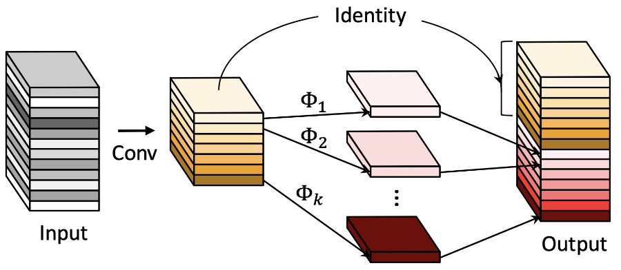
Figure taken from the paper.
First there is a regular convolution but with relatively few filters. It can have any kernel size you want. Because this convolution has a limited number of filters, it only generates a small number of feature maps (the yellow-orange ones).
Next, a series of inexpensive linear operations (shown in the image as ɸ) is used to create “ghost” features from the convolution’s output. One original feature map can be used to create multiple of these ghost feature maps (the pink-red ones).
The ghost feature maps are concatenated with the unmodified feature maps to create the final output tensor for this Ghost module. (This can be implemented by making one of the ɸ operations the identity function.)
The reason this technique works, is that in large neural networks, many of the feature maps generated by a convolution layer are redundant, i.e. they are very much alike. This is actually a good thing (see CondenseNet). The Ghost module simply creates these redundant feature maps in a more cost-efficient way.
Now, what exactly are these linear operations? Guess what: depthwise convolution. Yup, the ɸ is nothing more than a depthwise convolution layer.
The paper’s authors also experimented with affine and wavelet transformations, but depthwise convolution is fast and can learn to do many linear operations such as smoothing, finding edges, and so on.
So, despite the fancy name, a Ghost module is just a regular convolution followed by a depthwise convolution. (There usually wouldn’t be an activation function in between these two.)
It’s possible to use the Ghost module as a drop-in replacement for conv layers in existing architectures. Generally, this will increase the accuracy and lower the FLOPS. But the paper also describes GhostNet, an efficient architecture based on Ghost modules.
GhostNet is made up of the Ghost bottleneck. This is a building block consisting of two Ghost modules in a row with ReLU between them, plus a residual connection. The first Ghost module expands the number of channels, the second one reduces them again. There is also a strided version that puts a depthwise convolution with stride 2 in between the two Ghost modules.
In the Ghost modules used by GhostNet, the ordinary convolution has kernel size 1×1, while the depthwise convolutions for the linear transformations use kernel size 3×3. For each original feature map, this generates one new ghost feature map.
Note: I find it interesting that the regular convolution is a 1×1 layer here. Normally this would be something like 3×3 so that it has some kind of receptive field. Here, this convolution layer doesn’t actually do any filtering, only the depthwise layer (ɸ) does that. It’s kind of like an upside-down MobileNet v1 block.
The overall architecture of GhostNet follows MobileNet v3, but of course the blocks are now Ghost bottlenecks. (They also sometimes use squeeze-and-excitation, but not hard-swish.)
ImageNet classification accuracy:
| parameters | top-1 | top-5 | |
|---|---|---|---|
| GhostNet 0.5× | 2.6 M | 66.2% | 86.6% |
| GhostNet 1.0× | 5.2 M | 73.9% | 91.4% |
| GhostNet 1.3× | 7.3 M | 75.7% | 92.7% |
The paper claims they beat MobileNet v3. I’d say it’s about even when you take the number of parameters into account.
Speed test (in seconds):
| CPU | GPU | ANE | |
|---|---|---|---|
| iPhone 11 | 0.0127 | 0.0143 | 0.0119 |
| iPhone XS | 0.0134 | 0.0203 | 0.0184 |
| iPhone X | 0.0173 | 0.0266 | n/a |
Measurements are for GhostNet 1.0×. It’s a little faster than MobileNet v3 (large).
Conclusion: This did better than I expected in the speed department. But as with MobileNet v3, Core ML only runs a portion of this model on the ANE, the rest gets passed off to the GPU. So it’s not able to take full advantage of the Neural Engine (again due to the SE layers, I expect).
MixNet (2019)
Paper: MixConv: Mixed Depthwise Convolutional Kernels
Source code and checkpoints: TensorFlow TPU
The idea: Experimentation shows that the kernel size of depthwise convolution matters. But which size is the best? So, let’s try all of them! This paper introduces a new layer, MixConv, that puts multiple kernel sizes in a single convolution layer.
Many architectures use 3×3 kernels in their depthwise convolutions. Some of the newer ones also use 5×5 kernels or even 7×7. Up to a certain point, larger kernels improve accuracy — at the cost of more parameters and lower latency — but, as this paper shows, when the kernel becomes larger than 9×9 the accuracy actually gets worse.
The idea behind MixConv is simple: split up the channels into groups and apply a depthwise convolution with a different kernel size to each group.
This is a bit like an Inception module except it happens inside a single convolution layer. In practice, MixConv is implemented in three stages:
- Split the tensor into
Ggroups along the channel dimension. - Perform a different depthwise convolution on each group.
- Concatenate the results along the channel dimension again.
Typically, MixConv uses a value for G that is between 1 and 5. The convolution for the i-th group uses kernel size 2i + 1. For example, with three groups, the kernel sizes are 3×3, 5×5, and 7×7. (If G is 1, the layer acts as a regular 3×3 depthwise convolution.)
The obvious thing to do is to split up the tensor in groups of equal size, but the paper also experiments with another method where larger kernels get a smaller number of channels.
MixConv can be used as a drop-in replacement for depthwise convolution. The paper shows that using it in MobileNet v1 or v2 will boost the accuracy at the cost of adding just a few parameters when compared to 3×3 convolution.
But why stop there? These days, you stick it in a neural architecture search (NAS) and see if you can discover an architecture that works really well. They used similar settings to MnasNet and FBNet, but in addition to the usual search space based on MobileNet v2 blocks, it also includes MixConv layers.
This is what the architecture of MixNet-S looks like:
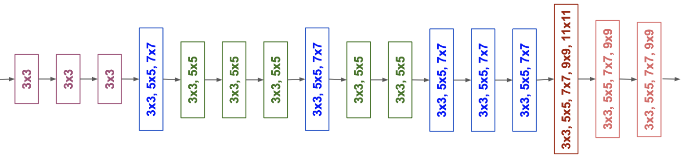
Based on the figure from the paper.
As you can see, not all layers use MixConv. It’s clear that the architecture search prefers smaller kernels in the early layers (to save computational cost) and larger kernels in the later layers (for better accuracy).
There is also one layer that uses very large kernels. Apparently using 11×11 with a regular depthwise layer gives pretty bad results, but inside a MixConv layer it works much better.
ImageNet classification accuracy:
| parameters | top-1 | top-5 | |
|---|---|---|---|
| MixNet-S | 4.1 M | 75.8% | 92.8% |
| MixNet-M | 5.0 M | 77.0% | 93.3% |
| MixNet-L | 7.3 M | 78.9% | 94.2% |
Nice! These scores are significantly better than other models of similar sizes.
Speed test (in seconds):
| CPU | GPU | ANE | |
|---|---|---|---|
| iPhone 11 | 0.0322 | 0.0392 | 0.0438 |
| iPhone XS | 0.0375 | 0.0532 | 0.0549 |
| iPhone X | 0.0528 | 0.0674 | n/a |
Measurements are for MixNet-M.
Conclusion: I didn’t think this would be fast. There is no native MixConv layer in Core ML. This is implemented by first splitting the tensor, then running multiple depthwise convolutions in parallel, and finally concatenating the results. That’s obviously going to slow things down.
EfficientNet (2019, 2020)
Paper: EfficientNet: Rethinking Model Scaling for Convolutional Neural Networks
Source code and checkpoints: TensorFlow TPU
The pièce de résistance. EfficientNet is rapidly replacing ResNet as the backbone of choice for many deep learning tasks. It’s at the top of the ImageNet classification leaderboards.
The idea: Many of the models in this blog post have a “multiplier” of some kind that lets you determine how many filters each layer has. A smaller multiplier makes the model faster, a larger multiplier makes the model more accurate. But that’s not the only way to scale a convnet.
There are actually three different things that can be scaled up or down:
Network width: How many filters there are per convolution layer. This is the one I just mentioned.
Network depth: How many layers there are in each stage of the model. The number of stages stays the same, but stages can be made deeper by adding more layers to them.
Input resolution: The dimensions of the input image. It’s common to use 224×224 images, but making the resolution higher will generally improve the accuracy (up to a point).
Note: Sometimes people use the term “depth multiplier” when they mean “width multiplier”. They’re talking about the depth of a single layer, i.e. how many filters it has. I think “channel” or “filter” multiplier would have been a better term. In the case of EfficientNet, the depth multiplier really determines how deep the model is, i.e. how many layers it has.
Tip: Even if a model is trained with a certain input resolution, you can often use smaller images at runtime. For example, using 128×224 instead of 224×224 will give the model a nice speed boost, plus it keeps the 16:9 aspect ratio of the camera so you don’t have to crop or pad the image.
It turns out that for effectively scaling a neural network up or down, you need to balance these three things as they all depend on each other. As the EfficientNet paper puts it,
“Intuitively, … if the input image is bigger, then the network needs more layers to increase the receptive field and more channels to capture more fine-grained patterns on the bigger image.”
The paper explores a new scaling method, compound scaling, that lets you scale the network’s depth, width, and input resolution together. The goal is to achieve the maximum possible accuracy while using as few FLOPS as possible.
To make this scaling method easy to use in practice, you just choose a single scaling factor \(\phi\). Then, the amount of scaling needed for depth, width, and input resolution is derived from this as follows:
- the network depth is scaled by \(\alpha^\phi\),
- the width by \(\beta^\phi\),
- and the resolution by \(\gamma^\phi\).
The values of \(\alpha, \beta, \gamma\) are fixed. In the paper they used grid search to come up with \(\alpha = 1.2, \beta = 1.1, \gamma = 1.15\). These values are chosen such that for any new \(\phi\), the total FLOPS will increase by \(2^\phi\) (approximately).
First, they use neural architecture search to find a baseline network. This is named EfficientNet-B0. It’s very similar to MnasNet and uses the same MBConv building blocks with 3×3 and 5×5 depthwise convolutions, squeeze-and-excitation (SE), and swish activation. There is nothing particularly new in this architecture.
The achitecture for EfficientNet-B0 looks like this:
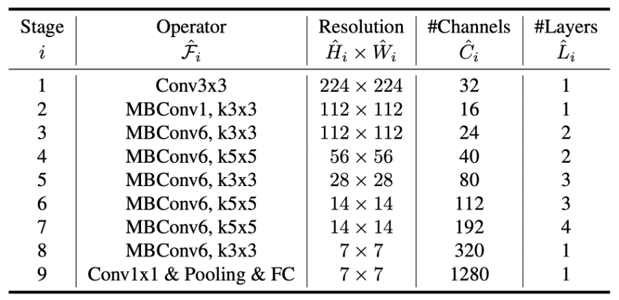
Figure taken from the paper.
EfficientNet-B0 is the smallest model (\(\phi = 1\) ). Next, they vary \(\phi\) to scale this model up, which gives EfficientNet-B1 to B7. For all these models, the number of stages and the types of building blocks stay the same (\(\mathcal{F}\) in the above table), but \(H \times W\) (resolution), \(C\) (width), and \(L\) (depth) all become larger.
EfficientNet-B0 has about 5 million parameters, so it’s already a fairly small model. But there are also special versions of EfficientNet that target smaller devices.
First, let’s look at EfficientNet-EdgeTPU (source code, blog post).
The EdgeTPU is Google’s version of the Neural Engine. Using architecture search, they tuned EfficientNet to give good performance on EdgeTPUs. For example, depthwise convolutions were sometimes replaced again by plain old convolutions because it turned out this was actually faster! 🤯
They also removed swish activation and squeeze-and-excitation (SE), because the EdgeTPU does not naturally support such operations — as we’ve seen, the same appears to be true for the Neural Engine.
Like before, they start with a baseline model, EfficientNet-EdgeTPU-S, and then use the compound scaling method to produce larger versions (M and L).
Finally, there is EfficientNet-Lite (source code, blog post).
This “lite” version of EfficientNet was released literally while I was writing this blog post, so good timing I guess. 😆 The Lite model is not optimized just for EdgeTPU, it’s also supposed to run well on mobile CPU and GPU.
As with the Edge models, EfficientNet-Lite does not have SE. Swish is replaced by ReLU6, mostly because this makes it easier to quantize the model weights.
According to the release notes, they also “Fixed the stem and head while scaling models up in order to reduce the size and computations of scaled models.” I’m not sure exactly what they did there but I assume it’s similar to MobileNet v3, which simplified the first and last layers in the model, as these are relatively expensive.
There are five versions: EfficientNet-Lite0 through Lite4, where 0 is the smallest and 4 is the largest. As is true for all EfficientNet models, the larger ones were made by scaling up the baseline model.
Note: Worth mentioning are some other variations of EfficientNet.
CondConv: Conditionally Parameterized Convolutions for Efficient Inference introduces a new layer, CondConv, which boosts EfficientNet accuracy by a few percentage points. The convolution kernel now has different sets of weights, and which weights it uses depends on the input tensor. Interesting idea, but the runtime cost of doing this probably isn’t worth the accuracy gains.
Adversarial Examples Improve Image Recognition describes EfficientNet-B8, an extra large model that is trained using adversarial examples.
Self-training with Noisy Student improves ImageNet classification introduces EfficientNet-L2 and trains it using pseudo labels on a huge dataset. EfficientNet models trained with this method are at the top of the ImageNet leaderboard right now, with top-1 accuracies of over 88% and top-5 over 98%. Impressive, but way outside the scope of mobile usage.
ImageNet classification accuracy:
| parameters | top-1 | top-5 | |
|---|---|---|---|
| EfficientNet-B0 | 5.3 M | 77.3% | 93.5% |
| EfficientNet-B1 | 7.8 M | 79.2% | 94.5% |
| EfficientNet-B0 (NoisyStudent) | 5.3 M | 78.7% | 94.4% |
| EfficientNet-B1 (NoisyStudent) | 7.8 M | 81.4% | 95.7% |
| EfficientNet-EdgeTPU-Small | 5.4 M | 77.2% | 93.6% |
| EfficientNet-EdgeTPU-Medium | 6.8 M | 78.7% | 94.3% |
| EfficientNet-EdgeTPU-Large | 10.5 M | 80.4% | 95.2% |
| EfficientNet-Lite0 | 4.7 M | 74.8% | 92.2% |
| EfficientNet-Lite1 | 5.4 M | 76.6% | 93.2% |
| EfficientNet-Lite2 | 6.1 M | 77.5% | 93.7% |
| EfficientNet-Lite3 | 8.2 M | 79.8% | 94.9% |
| EfficientNet-Lite4 | 13.0 M | 81.5% | 95.7% |
I did not include larger versions because those have many more parameters and therefore are unsuitable for mobile.
Except for the smallest Lite model, all these models score better than ResNet-50 and have way fewer parameters and FLOPS. Pretty impressive.
Notice that the Lite models have less accuracy than the regular ones for the same number of parameters. This makes it clear that squeeze-and-excite and swish definitely have a positive impact on accuracy, but also that they’re not worth it on mobile right now.
Note: The larger the EfficientNet model, the larger the input image is expected to be. For B0 and Lite0 it is 224×224 pixels, for B1 and Lite1 it is 240×240, and so on. For the largest model, B7, it is 600×600 pixels.
Speed test (in seconds):
| CPU | GPU | ANE | ||
|---|---|---|---|---|
| EfficientNet-B0 | iPhone 11 | 0.0309 | 0.0260 | 0.0253 |
| iPhone XS | 0.0363 | 0.0365 | 0.0353 | |
| iPhone X | 0.0478 | 0.0461 | n/a | |
| EfficientNet-Lite0 | iPhone 11 | 0.0245 | 0.0233 | 0.0065 |
| iPhone XS | 0.0303 | 0.0342 | 0.0089 | |
| iPhone X | 0.0369 | 0.0435 | n/a |
Unsurprisingly, EfficientNet-B0 is not able to use the Neural Engine to the fullest because SE involves a broadcasted multiply. Lite does not have SE and is therefore way faster on the ANE.
Conclusion: For CPU and GPU, the speed difference between B0 and Lite is small, so you might as well use B0 for the slightly better accuracy. But if your plan is to use the Neural Engine, you’ll definitely want to choose one of the Lite versions.
The end
So… if you’re building a new model for use on iPhone or iPad, which architecture should you use for your backbone?
I’ve been a big fan of MobileNet v1 and v2, and I still think these are good options. Unfortunately, v3 is a little bit of a let-down because of its bad performance on the Neural Engine.
Many other of the new models have disappointing results on the ANE as well.
EfficientNet is one of the best scoring models, and I expect many people will start using this because of the buzz surrounding it. Speedwise, I’m not impressed — it’s not the slowest model but it’s also not the fastest.
My conclusion at this point is that:
- MobileNet v3 is the best option for the CPU and GPU.
- FBNet-C is the best option for the Neural Engine.
These two choices give a nice trade-off between accuracy and speed. If you want more accuracy at the cost of slightly slower results, pick EfficientNet-Lite.
First published on Wednesday, 8 April 2020.
If you liked this post, say hi on Twitter @mhollemans or LinkedIn.
Find the source code on my GitHub.
 New e-book: Code Your Own Synth Plug-Ins With C++ and JUCE
Interested in how computers make sound? Learn the fundamentals of audio programming by building a fully-featured software synthesizer plug-in, with every step explained in detail. Not too much math, lots of in-depth information! Get the book at Leanpub.com