Getting started with TensorFlow on iOS

Before you can use a deep learning network to make predictions, you first have to train it. There are many different tools for training neural networks but TensorFlow is quickly becoming the weapon of choice for many.

You can use TensorFlow for training your machine learning models and for making predictions using those models. Training is usually done on a powerful machine or in the cloud, but TensorFlow also works on iOS — albeit with some limitations.

In this blog post I’ll explain the ideas behind TensorFlow, how to use it to train a simple classifier, and how to put this classifier in your iOS apps.

We’ll be using the Gender Recognition by Voice and Speech Analysis dataset to learn how to identify a voice as male or female based on audio recordings.

Get the code: You can find the source code for this project on GitHub.

What is a TensorFlow and why do I need one?

TensorFlow is a software library for building computational graphs in order to do machine learning.

Many other tools work at a higher level of abstraction. With Caffe for example, you design a neural network by connecting different kinds of “layers”. This is similar to the functionality that BNNS and MPSCNN provide on iOS.

In TensorFlow you can also work with such layers but you can go much deeper too, all the way down to the individual computations that make up your algorithm.

You can think of TensorFlow as a toolkit for implementing new machine learning algorithms, while other deep learning tools are for using algorithms implemented by other people.

That doesn’t mean you always have to build everything from scratch. TensorFlow comes with a collection of reusable building blocks, and there are other libraries such as Keras that provide convenient modules on top of TensorFlow.

So going deep into the math is not a requirement of using TensorFlow, but the option is there if you want to get your hands dirty.

Binary classification with logistic regression

In this blog post, we’ll create a classifier using the logistic regression algorithm. And yes, we’ll be building it from the ground up. So roll up those sleeves!

A classifier takes in some input data and then tells you which category — or class — this data belongs to. For this project we only have two classes: male or female, and therefore ours is a binary classifier.

The input data we’ll use consists of 20 numbers that represent various acoustic properties of a particular recording of someone speaking. I’ll explain more about this later but think of audio frequencies and that kind of information.

In the diagram below you can see that those 20 numbers are connected to a little block called sum. The connections have different weights, which correspond to how important each of these 20 numbers is, according to the classifier.

This is the block diagram of how a logistic classifier operates:

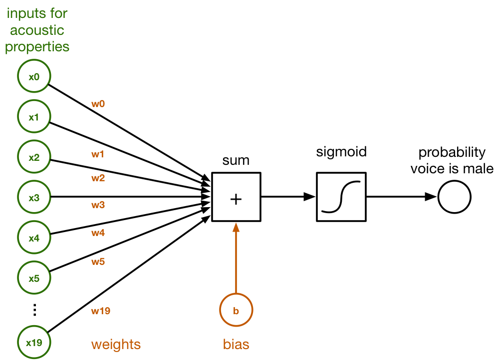
Inside the sum block, the inputs given by x0 – x19 and the weights of their connections w0 – w19 are simply summed up. This is a regular dot product:

sum = x[0]*w[0] + x[1]*w[1] + x[2]*w[2] + ... + x[19]*w[19] + b

We also add a so-called bias term b at the end. This is just another number.

The weights in the array w and the value of b represent what the classifier has learned. Training the classifier is a matter of finding the right numbers for w and b. Initially, we’ll start out with all w’s and b being zero. After many rounds of training, w and b will contain a set of numbers that the classifier can use to tell apart male speech from female speech.

To convert this sum into a probability, which is a number between 0 and 1, we apply the logistic sigmoid function:

y_pred = 1 / (1 + exp(-sum))

This formula may look scary but what it does is simple: if sum is a large positive number, the sigmoid function returns 1 or a probability of 100%. If sum is a large negative number, the sigmoid function returns 0. So for large positive or negative numbers, we get a confident “yes” or “no” prediction.

However, if sum is close to 0, the sigmoid function gives a probability closer to 50% because it is unsure about the prediction. When we start training the classifier, the initial predictions will be 50 / 50 because the classifier hasn’t learned anything yet and is not confident at all about the outcome. But the more we train, the more the probabilities tend to 1 and 0, and the more certain the classifier becomes.

Now y_pred contains the predicted outcome, the probability that the speech was from a male voice. If it is more than 0.5 (or 50%), we conclude the voice was male, otherwise it was female.

And that’s the idea behind doing binary classification using logistic regression. The input to the classifier consists of 20 numbers that describe acoustic features of an audio recording, we compute a weighted sum and apply the sigmoid function, and the output we get is the probability the speaker is male.

However, we still need to build the mechanics for training the classifier, and for that we turn to TensorFlow.

Implementing the classifier in TensorFlow

To use the classifier in TensorFlow, we need to turn its design into a computational graph first. A computational graph consists of nodes that perform calculations, and of the data that flows between these nodes.

The graph for our logistic regression looks like this:

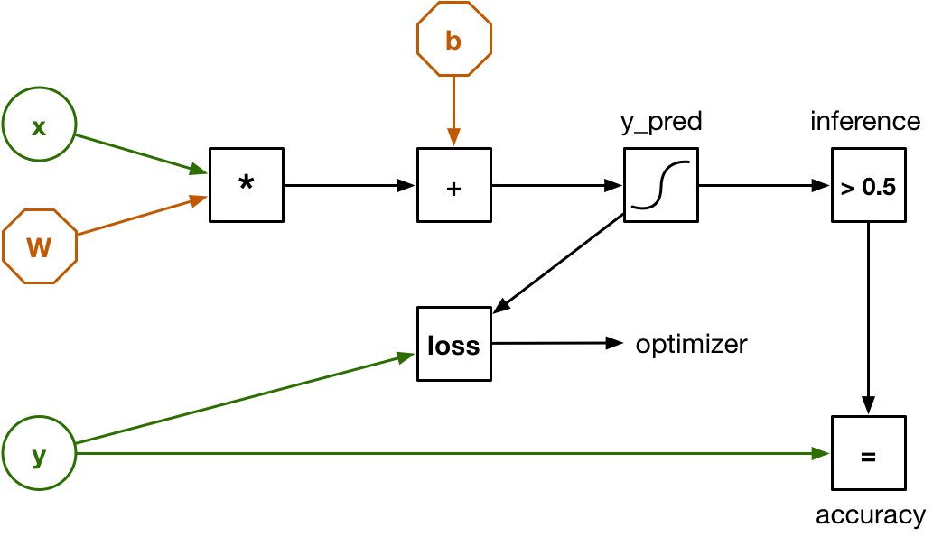
This looks a bit different than the earlier diagram, but that’s because the input x is no longer 20 separate numbers but a vector with 20 elements inside it. The weights are represented by a matrix W. So the dot product from before has been replaced by a single matrix multiplication.

There is also an input y. This is used for training the classifier and for verifying how well it works. The dataset we’re using has 3,168 examples of recorded speech, and for each example we also know whether it was made by a male voice or a female voice. Those known outcomes — male or female — are also called the labels of the dataset and that is what we’ll put into y.

To train the classifier, we load one of the examples into x and let the graph make a prediction: is it male or is it female? Because the weights are all zero initially, the classifier will likely make the wrong prediction. We need a way to calculate just “how much” wrong it is, and that is done by the loss function. The loss function compares the predicted outcome y_pred with the correct outcome y.

Given the loss for the training example, we use a technique called backpropagation to go backwards through the computational graph to adjust the weights W and b slightly in the right direction. If the prediction was male but the correct answer was female, the weights are shifted up or down a little so that next time the outcome “female” will be more likely for this particular input.

This training procedure is repeated for all examples from the data set, over and over and over, until the graph settles on an optimal set of weights. The loss, which measures how wrong the predictions are, consequently becomes lower over time.

Backpropagation is a great technique for training these kinds of computational graphs but the math involved can be a little tricky to get right. Here is the cool thing about TensorFlow: since we expressed all the “forward” operations as nodes in a graph, it can automatically figure out what the “backward” operations are for doing backpropagation — you don’t have to do any of that math yourself. Sweet!

So what is a tensor anyway?

In the graph above the data flows from left to right, from inputs to outputs. That’s the “flow” part of TensorFlow’s name. But what is a tensor?

All the data flowing through the graph is in the form of tensors. A tensor is just a cool name for an n-dimensional array. I said that W is a matrix of weights but as far as TensorFlow is concerned it really is a second-order tensor — in other words, a two-dimensional array.

• a scalar number is a zeroth-order tensor
• a vector is a first-order tensor
• a matrix is a second-order tensor
• a three-dimensional array is a third-order tensor
• and so on…

That’s all there is to it. With deep learning such as convolutional neural networks you’re often dealing with tensors of four dimensions, but our logistic classifier is much simpler and so we won’t go beyond second-order tensors, a.k.a matrices.

I also said x was a vector — or a first-order tensor if you want — but we’re going to treat it as a matrix too. The same thing is true for y. This lets us compute the loss over the entire dataset in one go.

A single example has 20 data elements. If we load all 3,168 examples into x, then x becomes a 3168×20 matrix. After multiplying x with W, the outcome y_pred is a 3168×1 matrix. That is, y_pred has one prediction for each of the examples in the dataset.

By expressing our graph in terms of matrices/tensors, we can make predictions for many examples at once.

Installing TensorFlow

OK, that’s the theory, now let’s put it into practice.

We’ll be using TensorFlow with Python. Your Mac may already have a version of Python installed but it may be an old version. I’m using Python 3.6 for this tutorial, so it’s best if you install that too.

Installing Python 3.6 is easiest using the Homebrew package manager. If you don’t have homebrew installed yet, first follow these instructions.

Then open a Terminal and type the following command to install the latest version of Python:

brew install python3

Python comes with its own package manager, pip, and we’ll use that to install the packages we need. From the Terminal, do the following:

pip3 install numpy
pip3 install scipy
pip3 install scikit-learn
pip3 install pandas
pip3 install tensorflow

In addition to TensorFlow we’ll also install NumPy, SciPy, pandas, and scikit-learn:

• NumPy is a library for working with n-dimensional arrays. Sound familiar? NumPy doesn’t call them tensors, but it’s the same thing. The TensorFlow Python API is built on top of NumPy.

• SciPy is a library for numerical computing. It is used by some of these other packages.

• pandas is useful for loading datasets and cleaning them up.

• scikit-learn is in some ways a competitor to TensorFlow, as it is a library for machine learning. We’re using it for our project because it has a number of handy functions. Since both TensorFlow and scikit-learn use NumPy arrays they can work together well.

You don’t necessarily need pandas and scikit-learn to use TensorFlow, but they are convenient and belong in any data scientist’s toolbox.

Just so you know, these packages will be installed in /usr/local/lib/python3.6/site-packages. This is useful in case you need to look something up in the TensorFlow source code that isn’t documented on the website.

Let’s do a quick test to make sure everything is installed correctly. Create a new text file tryit.py with the following contents:

import tensorflow as tf

a = tf.constant([1, 2, 3])
b = tf.constant([4, 5, 6])

sess = tf.Session(config=tf.ConfigProto(log_device_placement=True))

print(sess.run(a + b))

Then run this script from the Terminal:

python3 tryit.py

It will output some debugging information about the device TensorFlow is running on (most likely the CPU but possibly a GPU if you have a Mac with an NVIDIA GPU). At the end it should say,

[5 7 9]

which is the sum of the two vectors a and b.

It is possible that you also see messages such as:

W tensorflow/core/platform/cpu_feature_guard.cc:45] The TensorFlow library 
wasn't compiled to use SSE4.1 instructions, but these are available on your 
machine and could speed up CPU computations.

If this happens the version of TensorFlow that was installed on your system is not the most optimal for your CPU. One way to fix this is to build TensorFlow from source, because that lets you configure all the options. But for now it’s not a big deal if you see those warnings.

Taking a closer look at the data

To train a classifier, you need data.

For this project we’re using the “Gender Recognition by Voice” dataset from Kory Becker. I wanted to do something other than the usual MNIST digit recognition that you see in TensorFlow tutorials, so I went on Kaggle.com to look for a dataset and this one looked interesting.

So how do you recognize voice from audio? If you download the dataset and look inside the voice.csv file you’ll just see rows and rows of numbers:

It’s important to realize that this is not actual audio data! Instead, these numbers represent different acoustic properties of recorded speech. These properties — or features — were extracted from the audio recordings by a script and turned into this CSV file. Exactly how this was done is outside the scope of this tutorial, but if you’re interested you can consult the original R source code.

The dataset contains 3,168 of such examples (one for each row in the spreadsheet), roughly half from male speakers and half from female speakers. For each example there are 20 acoustic features, such as:

• the mean frequency in kHz
• the standard deviation of the frequency
• spectral flatness
• spectral entropy
• kurtosis
• maximum fundamental frequency measured across acoustic signal
• modulation index
• and so on…

For most of these I have no idea what they mean, and it’s not really important. All we care about is that we can use this data to train a classifier so that it can tell male and female voices apart, given these features.

If you wanted to use this classifier in an app to detect the gender of speech from an audio recording or audio from the microphone, you will first have to extract these acoustic properties from the audio data. Once you have those 20 numbers you can then give them to the trained classifier and it will tell you whether the voice is male or female.

So our classifier won’t work directly on an audio recording, only on the features that you extract from the recording.

Creating a training set and test set

Earlier I mentioned that we train the classifier by:

1. feeding it all the examples from the dataset,
2. measuring how wrong the predictions are,
3. and adjusting the weights based on the loss.

It turns out we shouldn’t use all of the data for training. We need to keep apart a portion of the data — known as the test set — so that we can evaluate how well our classifier works. So we will split up the dataset into two parts: the training set that we use to train the classifier, and the test set that we use to see how accurate the classifier is.

To split up the data into training and test sets, I created a Python script called split_data.py. This is what it looks like:

import numpy as np               # 1
import pandas as pd

df = pd.read_csv("voice.csv", header=0)        # 2

labels = (df["label"] == "male").values * 1    # 3
labels = labels.reshape(-1, 1)                 # 4

del df["label"]                  # 5
data = df.values

# 6
from sklearn.model_selection import train_test_split
X_train, X_test, y_train, y_test = train_test_split(data, labels,
                                       test_size=0.3, random_state=123456)

np.save("X_train.npy", X_train)  # 7
np.save("X_test.npy", X_test)
np.save("y_train.npy", y_train)
np.save("y_test.npy", y_test)

Step-by-step, here’s how this script works:

1. Import the NumPy and pandas packages. Pandas makes it really easy to load CSV files and do preprocessing on the data.
2. Use Pandas to load the dataset from voice.csv into a so-called dataframe. This object works very much like a spreadsheet or an SQL table.
3. The label column contains the labels for the dataset: whether an example is male or female. Here we extract the labels into a new NumPy array. The original labels are text but we convert this to numbers where 1 = male, 0 = female. (The assignment of those numbers is arbitrary — in a binary classifier we often use 1 to mean the “positive” class, or the class that we’re trying to detect.)
4. The new labels array is a one-dimensional array but our TensorFlow script will expect a two-dimensional tensor of 3,168 rows where each row has one column. So here we “reshape” the array to become two-dimensional. This doesn’t change the data in memory, only how NumPy interprets this data from now on.
5. Once we’re done with the label column we remove it from the dataframe, so that we’re left with the 20 features that describe the input. We also convert the dataframe into a regular NumPy array.
6. We use a helper function from scikit-learn to split the data and labels arrays into two portions. This randomly shuffles the examples in the dataset based on random_state, which is the seed for the random generator. It doesn’t matter what this seed it, but by always using the same seed we create a reproducible experiment.
7. Finally, save the four new arrays in NumPy’s binary file format. We now have a training set and a test set!

You can do additional preprocessing on the data in this script — such as scaling the features so they have zero mean and identical variance — but I left that out for this simple project.

Run the script from Terminal like so:

python3 split_data.py

This gives us four new files that contain the training examples (X_train.npy) and the labels for those examples (y_train.npy), as well as the test examples (X_test.npy) and their labels (y_test.npy).

Building the computational graph

Now that we have the data sorted out, we can write a script for training the logistic classifier with TensorFlow. This script is called train.py. To save space I won’t show the entire script here, you can see it on GitHub.

As usual, we first import the packages we need. And then we load the training data into two NumPy arrays: X_train and y_train. (We’re not using the test data in this script.)

import numpy as np
import tensorflow as tf

X_train = np.load("X_train.npy")
y_train = np.load("y_train.npy")

Now we can build our computational graph. First we define so-called placeholders for our inputs x and y:

num_inputs = 20
num_classes = 1

with tf.name_scope("inputs"):
    x = tf.placeholder(tf.float32, [None, num_inputs], name="x-input")
    y = tf.placeholder(tf.float32, [None, num_classes], name="y-input")

The tf.name_scope("...") is useful for grouping different parts of the graph into different scopes, which makes it easier to understand the graph. We put x and y inside the "inputs" scope. We also give them names, "x-input" and "y-input", so we can easily refer to them later on.

Recall that each input example is a vector of 20 elements. Each example also has a label (1 is male, 0 is female). I also mentioned that we can compute everything in one go if we combine all the examples into a matrix. That’s why x and y are defined as two-dimensional tensors here: x has dimensions [None, 20] and y has dimensions [None, 1].

The None means that the first dimension is flexible and not known yet. In case of the training set we’ll put 2,217 examples into x and y; in case of the test set it’s 951 examples.

Now that TensorFlow knows what our inputs are, we can define the classifier’s parameters:

with tf.name_scope("model"):
    W = tf.Variable(tf.zeros([num_inputs, num_classes]), name="W")
    b = tf.Variable(tf.zeros([num_classes]), name="b")

The tensor W contains the weights that the classifier will learn (a 20×1 matrix because there are 20 input features and 1 output) and b contains the bias value. These two are declared as TensorFlow variables, which means that they can be updated by the backpropagation procedure.

With all the pieces in place, we can declare the computation that is at the heart of our logistic regression classifier:

y_pred = tf.sigmoid(tf.matmul(x, W) + b)

This multiplies x and W, adds the bias b, and then takes the logistic sigmoid. The result in y_pred is the probability that the speaker of the audio data described by the features in x is male.

We’re not done yet. In order to train the model, we need to define a loss function. For a binary logistic regression classifier it makes sense to use the log loss, and fortunately TensorFlow has a built-in log_loss() function that saves us from writing out the actual math:

with tf.name_scope("loss-function"):
    loss = tf.losses.log_loss(labels=y, predictions=y_pred)
    loss += regularization * tf.nn.l2_loss(W)

The log_loss graph node takes as input y, the labels for the examples we’re currently looking at, and compares them to our predictions y_pred. This results in a number that represents the loss.

When we first start training, the prediction y_pred will be 0.5 (or 50% male) for all examples because the classifier has no idea yet what the right answer should be. The initial loss, computed as -ln(0.5), will therefore be 0.693146. As training progresses, the loss will become smaller and smaller.

The second line for computing the loss adds something called L2 regularization. This is done to prevent overfitting, to stop the classifier from exactly memorizing the training data. That won’t be much of an issue here, since our classifier’s “memory” only consists of 20 weight values and a bias value. But regularization is a common machine learning technique, so I thought I’d include it.

The regularization value is another placeholder:

with tf.name_scope("hyperparameters"):
    regularization = tf.placeholder(tf.float32, name="regularization")
    learning_rate = tf.placeholder(tf.float32, name="learning-rate")

We already used placeholders to define our inputs x and y, but they are also useful for defining hyperparameters. Hyperparameters let you configure the model and how it is trained. They’re called “hyper” parameters because unlike the regular parameters W and b they are not learned by the model — you have to set them to appropriate values yourself.

The learning_rate hyperparameter tells the optimizer how big of a steps it should take. The optimizer is what performs the backpropagation: it takes the loss and feeds it back into the graph to determine by how much to update the weights and bias values. There are many possible optimizers, but we’ll use ADAM:

with tf.name_scope("train"):
    optimizer = tf.train.AdamOptimizer(learning_rate)
    train_op = optimizer.minimize(loss)

This creates a node in the graph called train_op. This is the node we will “run” later on in order to train the classifier.

To determine how well the classifier is doing, we’ll take occasional snapshots during training and count how many examples from the training set it can correctly predict already. Accuracy on the training set is not a great indicator of how well the classifier works, but it’s useful to track anyway — if you’re training and the accuracy of predictions on the training set becomes worse, then something’s going wrong!

We define a graph node for computing the accuracy:

with tf.name_scope("score"):
    correct_prediction = tf.equal(tf.to_float(y_pred > 0.5), y)
    accuracy = tf.reduce_mean(tf.to_float(correct_prediction), name="accuracy")

We can run the accuracy node to see how many examples are correctly predicted. Recall that y_pred contains a probability between 0 and 1. By doing tf.to_float(y_pred > 0.5) we get a value of 0 if the prediction was female, and 1 if the prediction was male. We can compare that to y, which contains the correct values. The accuracy is then the number of correct predictions divided by the total number of predictions.

Later on we’ll also use this same accuracy node on the test set, to see how well the classifier really does.

It’s useful to define one more node. This one is used to make predictions on data for which we don’t have any labels at all:

with tf.name_scope("inference"):
    inference = tf.to_float(y_pred > 0.5, name="inference")

To use this classifier in an app you would record a few words of spoken text, analyze it to extract the 20 acoustic features, and then give those to the classifier. Because this is new data, not data from the training or test sets, you obviously won’t have a label for it. You can only give this new data to the classifier and hope that it predicts the correct result. That’s what the inference node is for.

OK, that was a lot of work just for building the computational graph. Now we want to actually train it on the training set.

Training the classifier

Training usually happens in an infinite loop. For this simple logistic classifier that’s a bit overkill — it takes less than a minute to train it — but for a deep neural network you want to let the script run for hours or days until the accuracy is good enough or you run out of patience.

Here’s the first part of the training loop in train.py:

with tf.Session() as sess:
    tf.train.write_graph(sess.graph_def, checkpoint_dir, "graph.pb", False)

    sess.run(init)

    step = 0
    while True:
    	# here comes the training code

First we create a new TensorFlow session object. To run the graph, you need a session. The call to sess.run(init) resets W and b to all zeros.

We also write the computational graph to a file. The serializes all the nodes that we just created into the file /tmp/voice/graph.pb. We need this graph definition later for running the classifier on the test set, but also for putting the trained classifier into the iOS app.

Inside the while True: loop, we do the following:

        perm = np.arange(len(X_train))
        np.random.shuffle(perm)
        X_train = X_train[perm]
        y_train = y_train[perm]

First, we randomly shuffle the training examples. This is important because you don’t want the classifier to inadvertently learn anything about the order that the examples happen to be in.

Next comes the important bit: we tell the session to run the train_op node. This will perform a single training run on the graph:

        feed = {x: X_train, y: y_train, learning_rate: 1e-2, 
                regularization: 1e-5}
        sess.run(train_op, feed_dict=feed)

When you say sess.run() you also need to provide a feed dictionary. This tells TensorFlow what the values of the placeholder nodes are.

Since this is a very simple classifier we always train on the entire training set at once, so we put the X_train array into placeholder x and the y_train array into placeholder y. (For larger datasets you would train in small batches of 100 to 1000 examples.)

And that’s all we need to do. Because we’re in an infinite loop, the train_op node is run many, many times. And on each iteration, the backpropagation mechanism makes a tiny change to the weights W and b. Over time, this causes the weights to settle on their optimal values.

It is useful to understand how the training is progressing, so we’ll print a progress report every so often (every 1000 steps in the demo project):

        if step % print_every == 0:
            train_accuracy, loss_value = sess.run([accuracy, loss], 
                                                  feed_dict=feed)
            print("step: %4d, loss: %.4f, training accuracy: %.4f" % \
                    (step, loss_value, train_accuracy))

This time we don’t run the train_op node but two other nodes: accuracy and loss. We use the same feed dictionary, so that the accuracy and loss are computed over the training set.

As I said before, a high training set accuracy doesn’t necessary mean the classifier will also do well on the test set, but you definitely want to see this number go up as training progresses. You should see the loss going down.

We’ll also save a checkpoint every so often:

        if step % save_every == 0:
            checkpoint_file = os.path.join(checkpoint_dir, "model")
            saver.save(sess, checkpoint_file)            
            print("*** SAVED MODEL ***")

This takes the values of W and b that the classifier has learned so far and saves them to a checkpoint file. This checkpoint is what we’ll read back in when we want to run the classifier on the test set. The checkpoint files are saved to the directory /tmp/voice/.

Run the training script from Terminal like so:

python3 train.py

The output should look something like this:

Training set size: (2217, 20)
Initial loss: 0.693146
step:    0, loss: 0.7432, training accuracy: 0.4754
step: 1000, loss: 0.4160, training accuracy: 0.8904
step: 2000, loss: 0.3259, training accuracy: 0.9170
step: 3000, loss: 0.2750, training accuracy: 0.9229
step: 4000, loss: 0.2408, training accuracy: 0.9337
step: 5000, loss: 0.2152, training accuracy: 0.9405
step: 6000, loss: 0.1957, training accuracy: 0.9553
step: 7000, loss: 0.1819, training accuracy: 0.9594
step: 8000, loss: 0.1717, training accuracy: 0.9635
step: 9000, loss: 0.1652, training accuracy: 0.9666
*** SAVED MODEL ***
step: 10000, loss: 0.1611, training accuracy: 0.9702
step: 11000, loss: 0.1589, training accuracy: 0.9707
. . .

Once you stop seeing the loss go down, wait until you see the next *** SAVED MODEL *** message and press Ctrl+C to stop training.

With the hyperparameter settings I’ve chosen for the regularization and learning rate, you should see a training set accuracy of about 97% and a loss of about 0.157. (If you set regularization to 0 in the feed dictionary, the loss will go even lower.)

How well does it do?

Once you’ve trained your classifier, you want to test it to see how well it really works in practice. You need to do this on data that was not used for training. This is why we split up the dataset into a training set and a test set.

We’ll create a new script, test.py, that loads the graph definition and the test set, and computes how many of the test examples it predicts correctly. I will only show you the relevant bits, the full script is here.

As before, the script first imports the packages, including the metrics package from scikit-learn to print out some additional reports. Of course, this time we load the test set instead of the training set.

import numpy as np
import tensorflow as tf
from sklearn import metrics

X_test = np.load("X_test.npy")
y_test = np.load("y_test.npy")

To compute the accuracy on the test set, we’ll need our computational graph again. Not the entire graph, because the nodes for training — train_op and loss — are not used now.

We could build up the graph by hand again but since we already saved it to the file graph.pb we might as well load it from that file. Here’s the code:

with tf.Session() as sess:
    graph_file = os.path.join(checkpoint_dir, "graph.pb")
    with tf.gfile.FastGFile(graph_file, "rb") as f:
        graph_def = tf.GraphDef()
        graph_def.ParseFromString(f.read())
        tf.import_graph_def(graph_def, name="")

TensorFlow likes to store its data as peanut butter protocol buffer files (hence the extension .pb), so we use some helper code to load this file and import it as a graph into the session.

Next, we need to load the values of W and b from the checkpoint file:

    W = sess.graph.get_tensor_by_name("model/W:0")
    b = sess.graph.get_tensor_by_name("model/b:0")

    checkpoint_file = os.path.join(checkpoint_dir, "model")
    saver = tf.train.Saver([W, b])
    saver.restore(sess, checkpoint_file)

This is why we put our nodes into scopes and gave them names, so we can easily find them again using get_tensor_by_name(). If you don’t give your nodes explicit names, then you have to dig through the graph definition to figure out what name TensorFlow assigned to it by default.

We also need to get references to a few other nodes, notably the inputs x and y and the nodes that make predictions:

    x = sess.graph.get_tensor_by_name("inputs/x-input:0")
    y = sess.graph.get_tensor_by_name("inputs/y-input:0")
    accuracy = sess.graph.get_tensor_by_name("score/accuracy:0")
    inference = sess.graph.get_tensor_by_name("inference/inference:0")

All right, so far all we’ve done is load the graph back into memory. We’ve also loaded what the classifier has learned into W and b again. Now we can finally test the accuracy of the classifier on data it has never seen before:

    feed = {x: X_test, y: y_test}
    print("Test set accuracy:", sess.run(accuracy, feed_dict=feed))

This runs the accuracy node with the acoustic features from the X_test array as input, and the labels from y_test for verification.

We can also show a few other reports, with the help of scikit-learn:

    predictions = sess.run(inference, feed_dict={x: X_test})
    print("Classification report:")
    print(metrics.classification_report(y_test.ravel(), predictions))
    print("Confusion matrix:")
    print(metrics.confusion_matrix(y_test.ravel(), predictions))

This time we’re using the inference node to get the predictions. Since inference just computes the predictions but does not check how accurate they are, the feed dictionary only has to include the input x but not y.

Run this script and you should see output similar to the following:

$ python3 test.py

Test set accuracy: 0.958991

Classification report:
             precision    recall  f1-score   support

          0       0.98      0.94      0.96       474
          1       0.94      0.98      0.96       477

avg / total       0.96      0.96      0.96       951

Confusion matrix:
[[446  28]
 [ 11 466]]

The accuracy on the test set is almost 96% — as expected a little lower than the training set accuracy, but it’s very close. That means our training was successful and we have verified that the classifier also works well on unseen data. It’s not perfect — 1 out of every 25 attempts will still be classified wrong — but it’s good enough for our purposes!

The classification report and confusion matrix show some statistics on which examples were wrongly predicted. From the confusion matrix we can tell that 446 of the female examples were correct but 28 of female examples were wrongly predicted to be male. Of the male examples 466 were identified correctly but 11 were misclassified as female.

So it seems that our classifier more often gets female voices wrong than it gets male voices wrong. The precision/recall figures from the classification report tell the same story.

TensorFlow on iOS

Now that we have a trained model that performs reasonably well on the test set, let’s build a simple iOS app that can use this model to make predictions. First, we’ll make an app that uses the TensorFlow C++ library. In the next section we’ll port the model to Metal for comparison.

There’s good news and there’s bad news. The bad news is that you’ll have to build TensorFlow from source. Actually, it gets worse: you need to install Java to do this. The good news is that it’s a fairly straightforward process. Full instructions are here but the following steps should work (tested on TensorFlow 1.0).

It goes without saying, but you should have Xcode 8 installed. Also make sure that the active developer directory points at your installation of Xcode (if you installed Homebrew before you installed Xcode, this may be pointing at the wrong place and TensorFlow won’t build):

sudo xcode-select -s /Applications/Xcode.app/Contents/Developer

TensorFlow is built using a tool called bazel, and bazel requires Java JDK 8. Installing the required packages is easy using Homebrew:

brew cask install java
brew install bazel
brew install automake
brew install libtool

Once that is done, you need to clone the TensorFlow GitHub repository. Important: do this in a path that doesn’t have spaces in it, otherwise bazel will refuse to build (yes, really!). I simply cloned to my home directory:

cd /Users/matthijs
git clone https://github.com/tensorflow/tensorflow -b r1.0

The -b r1.0 flag tells git to clone the r1.0 branch. Feel free to get a more recent branch (you can see the branches here) or the master branch if you feel like living on the edge.

Once the repo is cloned, you need to run the configure script.

cd tensorflow
./configure

This will ask a number of questions. Here is how I answered them:

Please specify the location of python. [Default is /usr/bin/python]:	

I answered with /usr/local/bin/python3 because I want to use Python 3.6 with TensorFlow. If you choose the default option then TensorFlow will be built with Python 2.7.

Please specify optimization flags to use during compilation [Default is 
-march=native]:

Just press Enter here. For the next couple of questions, choose n for no.

When it asks about which Python library to use, press Enter to choose the default (which should be the Python 3.6 library).

Answer the remaining questions with n for no. Now the script will download a number of dependencies and prepare everything for building TensorFlow.

Building the static library

There are two ways to build TensorFlow:

1. for your Mac, which uses the bazel build tool
2. for iOS, which uses a Makefile

We want to build for iOS, so we’ll go with option 2. However, we’ll also need to build some extra tools and that will involve option 1.

Execute the following script from within the tensorflow directory:

tensorflow/contrib/makefile/build_all_ios.sh

This first downloads a few dependencies and then it starts the build process. If all goes well, it will create three static libraries that need to be linked into your app: libtensorflow-core.a, libprotobuf.a, libprotobuf-lite.a.

We’re not done yet. There are two additional helper tools we need to build. From the Terminal, run the following two commands:

bazel build tensorflow/python/tools:freeze_graph
bazel build tensorflow/python/tools:optimize_for_inference

Note: This will take another 20 or so minutes as it will build TensorFlow again from scratch (this time using bazel).

Building TensorFlow for Mac

This step is optional but as you’ve installed all the prerequisite packages anyway, building TensorFlow for Mac is not difficult now. This creates a new pip package that you can install instead of the official TensorFlow package.

Why would you want to do this? Well, it lets you create a version of TensorFlow with custom options. For example, if you got the “The TensorFlow library wasn’t compiled to use SSE4.1 instructions” warnings while running the train.py script, you can compile a version of TensorFlow that enables these instructions.

To build TensorFlow for Mac, run the following from Terminal:

bazel build --copt=-march=native -c opt //tensorflow/tools/pip_package:build_pip_package

bazel-bin/tensorflow/tools/pip_package/build_pip_package /tmp/tensorflow_pkg

The -march=native option adds support for SSE, AVX, AVX2, FMA, etc instructions if they are available on your CPU.

Then to install the package:

pip3 uninstall tensorflow
sudo -H pip3 install /tmp/tensorflow_pkg/tensorflow-1.0.0-XXXXXX.whl

For more detailed instructions, see the TensorFlow website.

Freezing the graph

The iOS app we’ll be making will load the model that we trained with the Python script and uses it to make a few predictions.

Recall that train.py saved the graph definition to the file /tmp/voice/graph.pb. Unfortunately, you cannot load this graph as-is into the iOS app. The full graph contains operations that are not currently supported by the TensorFlow C++ API. That’s why we need to use the two extra tools we just built.

freeze_graph takes graph.pb and the checkpoint file that contains the trained values for W and b, and merges them into one file. It also removes any operations that are not supported on iOS.

Run this tool from a Terminal, from within the tensorflow directory:

bazel-bin/tensorflow/python/tools/freeze_graph \
--input_graph=/tmp/voice/graph.pb --input_checkpoint=/tmp/voice/model \
--output_node_names=model/y_pred,inference/inference --input_binary \
--output_graph=/tmp/voice/frozen.pb

This creates a simplified graph in /tmp/voice/frozen.pb that only has the nodes up to y_pred and inference. It does not include the nodes that are used for training.

The advantage of using freeze_graph is that it also sticks the weights into the file, so you don’t have to load these separately: frozen.pb contains everything we need.

The optimize_for_inference tool simplifies the graph even further. It takes as input the frozen.pb file and writes /tmp/voice/inference.pb as output. That is the file we’ll embed in the iOS app. Run the tool like so:

bazel-bin/tensorflow/python/tools/optimize_for_inference \
--input=/tmp/voice/frozen.pb --output=/tmp/voice/inference.pb \
--input_names=inputs/x --output_names=model/y_pred,inference/inference \
--frozen_graph=True

The iOS app

You can find the iOS app at github.com/hollance/TensorFlow-iOS-Example in the VoiceTensorFlow folder.

Open the project in Xcode. There are a few things to notice:

• The app is written in Objective-C++ (the source files end in .mm). At this point there is no Swift API for TensorFlow, only C++.
• The inference.pb file is already included in the project. You can copy your own version of inference.pb into the project folder if you want.
• The app links with Accelerate.framework.
• The app links with the static libraries you have just compiled.

Go to the Project Settings screen and switch to the Build Settings tab. Under Other Linker Flags you’ll see the following:

/Users/matthijs/tensorflow/tensorflow/contrib/makefile/gen/protobuf_ios/lib/
libprotobuf-lite.a 

/Users/matthijs/tensorflow/tensorflow/contrib/makefile/gen/protobuf_ios/lib/
libprotobuf.a 

-force_load /Users/matthijs/tensorflow/tensorflow/contrib/makefile/gen/lib/
libtensorflow-core.a

Unless your name is also “matthijs”, you will need to replace these with the path where you cloned the TensorFlow repository. (Notice that tensorflow appears twice, so the folder name is tensorflow/tensorflow/...)

Also check the Header Search Paths. These are currently set to:

~/tensorflow
~/tensorflow/tensorflow/contrib/makefile/downloads 
~/tensorflow/tensorflow/contrib/makefile/downloads/eigen 
~/tensorflow/tensorflow/contrib/makefile/downloads/protobuf/src 
~/tensorflow/tensorflow/contrib/makefile/gen/proto

Again, you have to update these to where you cloned the repository.

There are some other build settings that I changed from the defaults:

• Enable Bitcode: No
• Warnings / Documentation Comments: No
• Warnings / Deprecated Functions: No

Bitcode is not currently supported by TensorFlow, so I disabled that. I also turned off the warnings, otherwise you’d get loads of issues when you compile the app. (You will still get several Value Conversion Issue warnings. Feel free to disable those warnings too, but I personally like to be told about those.)

Once you have made the changes to the Other Linker Flags and the Header Search Paths, you can build and run the app.

Great, now you have an iOS app that uses TensorFlow! Let’s look at how it works.

Using the TensorFlow C++ API

TensorFlow for iOS is written in C++ but the amount of C++ code you need to write is — fortunately! — limited. Typically you’ll do the following:

1. load the graph and weights from a .pb file
2. create a session using that graph
3. put your data into an input tensor
4. run the graph on one or more nodes
5. get the results out of the output tensor

In the demo app, this all happens in ViewController.mm. First, we load the graph:

- (BOOL)loadGraphFromPath:(NSString *)path
{
    auto status = ReadBinaryProto(tensorflow::Env::Default(), 
                                  path.fileSystemRepresentation, &graph);
    if (!status.ok()) {
        NSLog(@"Error reading graph: %s", status.error_message().c_str());
        return NO;
    }
    return YES;
}

The Xcode project includes the graph inference.pb that we made by running the freeze_graph and optimize_for_inference tools on graph.pb. If you try to load graph.pb instead, you’ll get an error message:

Error adding graph to session: No OpKernel was registered to support Op 
'L2Loss' with these attrs.  Registered devices: [CPU], Registered kernels:
  <no registered kernels>

    [[Node: loss-function/L2Loss = L2Loss[T=DT_FLOAT](model/W/read)]]

The C++ API supports fewer operations than the Python API. Here it says that the L2Loss operation that we used in the loss function node is not available on iOS. That’s why we needed to use freeze_graph to simplify our graph.

After loading the graph, we can create a session:

- (BOOL)createSession
{
    tensorflow::SessionOptions options;
    auto status = tensorflow::NewSession(options, &session);
    if (!status.ok()) {
        NSLog(@"Error creating session: %s", 
                status.error_message().c_str());
        return NO;
    }

    status = session->Create(graph);
    if (!status.ok()) {
        NSLog(@"Error adding graph to session: %s", 
                status.error_message().c_str());
        return NO;
    }
    return YES;
}

Once we have the session we can use it to make some predictions. The predict: method takes an array of 20 floating point numbers — the acoustic features — and feeds these numbers into the graph.

Let’s take a look at how this method works:

- (void)predict:(float *)example {
    tensorflow::Tensor x(tensorflow::DT_FLOAT, 
                         tensorflow::TensorShape({ 1, 20 }));

    auto input = x.tensor<float, 2>();
    for (int i = 0; i < 20; ++i) {
        input(0, i) = example[i];
    }

This first defines the tensor x that we use for the input data. This tensor has shape {1, 20} because it takes one example at a time and that example has 20 features. Then we copy the data from the float * array into the tensor.

Next up we run the session:

    std::vector<std::pair<std::string, tensorflow::Tensor>> inputs = {
        {"inputs/x-input", x}
    };

    std::vector<std::string> nodes = {
        {"model/y_pred"},
        {"inference/inference"}
    };

    std::vector<tensorflow::Tensor> outputs;

    auto status = session->Run(inputs, nodes, {}, &outputs);
    if (!status.ok()) {
        NSLog(@"Error running model: %s", status.error_message().c_str());
        return;
    }

What happens here is analogous to the Python code,

    pred, inf = sess.run([y_pred, inference], feed_dict={x: example})

just not as succinct. We create the feed dictionary, as well as a vector that lists the nodes we want to run, and a vector that will hold the results. Finally, we tell the session to do its thing.

Once the session has run the nodes, we can print the results:

    auto y_pred = outputs[0].tensor<float, 2>();
    NSLog(@"Probability spoken by a male: %f%%", y_pred(0, 0));

    auto isMale = outputs[1].tensor<float, 2>();
    if (isMale(0, 0)) {
        NSLog(@"Prediction: male");
    } else {
        NSLog(@"Prediction: female");
    }
}

For our purposes it would be enough to just run the inference node to get a male/female prediction but I also wanted to see the computed probability, which is why we run the y_pred node too.

Running the app

You can run the app on the iPhone Simulator or on a device. On the simulator you may again get messages such as “The TensorFlow library wasn’t compiled to use SSE4.1 instructions”, but you shouldn’t get these on the device.

Just for testing purposes, the app will make two predictions: once for a male example and once for a female example. (I simply took those examples from the test set. Feel free to replace the numbers in the maleExample or femaleExample arrays with different examples.)

Run the app and you should see the following output. The app first prints out the nodes in the graph:

Node count: 9
Node 0: Placeholder 'inputs/x-input'
Node 1: Const 'model/W'
Node 2: Const 'model/b'
Node 3: MatMul 'model/MatMul'
Node 4: Add 'model/add'
Node 5: Sigmoid 'model/y_pred'
Node 6: Const 'inference/Greater/y'
Node 7: Greater 'inference/Greater'
Node 8: Cast 'inference/inference'

Notice how this graph only includes the operations needed to make predictions, it doesn’t have any of the training stuff.

Then it prints the results of the predictions:

Probability spoken by a male: 0.970405%
Prediction: male

Probability spoken by a male: 0.005632%
Prediction: female

If you try these same examples from a Python script, you will get the exact same answers. Mission successful!

Pros and cons of TensorFlow on iOS

TensorFlow is a great tool for training your machine learning models and, if you’re not afraid of some math, for implementing new algorithms. For training really big models you can even use TensorFlow in the cloud.

Besides training, this blog post has also shown how to add TensorFlow into your iOS apps. In this section, I want to summarize the pros and cons of doing so.

Advantages of using TensorFlow on iOS:

• Use one tool for everything. You can use TensorFlow both for training the model and for doing inference on the device. There is no need to port your computational graph to another API such as BNNS or Metal. On the other hand, you do need to “port” at least some of your Python code to C++.

• TensorFlow has many more features than BNNS or Metal.

• You can test it on the simulator. (Metal always needs to run on a device.)

Limitations of TensorFlow on iOS:

• Currently there is no GPU support. TensorFlow does use the Accelerate framework for taking advantage of CPU vector instructions, but when it comes to raw speed you can’t beat Metal.
• The TensorFlow API is C++, so you need to write your code in Objective-C++. You can’t directly use TensorFlow from Swift.
• The C++ API is more limited than the Python API. This means you cannot do training on the device, because the automatic gradient computation needed by backpropagation is not currently supported. This is not such a big deal right now, since mobile device hardware isn’t great for training on anyway.
• The TensorFlow static library adds about 40 MB to the size of the app bundle. You can make this smaller by reducing the number of supported operations, but that’s a big hassle. This does not include the size of your model, by the way, which may add many more megabytes.

Personally, I don’t think it’s worth the effort to use TensorFlow on iOS right now. The advantages don’t really outweigh the downsides. But it’s a young product, so who knows what TensorFlow has in store for the future…

Doing it on the GPU: using Metal

One of the downsides of using TensorFlow in your iOS app is that it runs on the CPU. For this particular project TensorFlow is more than adequate since the data and the model are so small. However, for larger models — and especially for deep learning — you want to use the GPU instead. And on iOS that means using Metal.

You’ll still do the training with TensorFlow on your Mac — or for big models on a Linux box with a fat GPU or even in the cloud — but the inference code that runs on iOS uses Metal instead of the TensorFlow library.

After training we need to export the learned parameters — the values of W and b — into a format that Metal can read. Fortunately, that just means saving them as a list of floating point numbers in binary format.

Time to write one more Python script: export_weights.py (full version here). This is very similar to test.py where we load the graph definition and the checkpoint. But this time we do:

    W.eval().tofile("W.bin")
    b.eval().tofile("b.bin")

W.eval() computes the current value of W and returns it as a NumPy array (it’s the same thing as doing sess.run(W)). Then we use tofile() to save the NumPy array to a binary file. And that’s all we need to do. :–)

Let’s look at the Metal version of our logistic classifier. You can find the Xcode project in the VoiceMetal folder of the source code. This project is written in Swift.

Recall that the logistic regression is computed by the formula:

y_pred = sigmoid((W * x) + b)

That’s exactly the same computation that a fully-connected layer from a neural network performs. So to implement our classifier with Metal, we just need to use an MPSCNNFullyConnected layer.

First we load W.bin and b.bin into Data objects:

let W_url = Bundle.main.url(forResource: "W", withExtension: "bin")
let b_url = Bundle.main.url(forResource: "b", withExtension: "bin")
let W_data = try! Data(contentsOf: W_url!)
let b_data = try! Data(contentsOf: b_url!)

Then we create the fully-connected layer:

let sigmoid = MPSCNNNeuronSigmoid(device: device)

let layerDesc = MPSCNNConvolutionDescriptor(
                   kernelWidth: 1, kernelHeight: 1, 
                   inputFeatureChannels: 20, outputFeatureChannels: 1, 
                   neuronFilter: sigmoid)

W_data.withUnsafeBytes { W in
  b_data.withUnsafeBytes { b in
    layer = MPSCNNFullyConnected(device: device, 
               convolutionDescriptor: layerDesc, 
               kernelWeights: W, biasTerms: b, flags: .none)
  }
}

Since the input is 20 numbers, I decided to make the fully-connected layer work on an “image” of dimensions 1×1 with 20 input channels. The result y_pred is a single number, so the fully-connected layer has only one output channel.

The input and output data are placed in MPSImage objects that also have those dimensions:

let inputImgDesc = MPSImageDescriptor(channelFormat: .float16, 
                       width: 1, height: 1, featureChannels: 20)
let outputImgDesc = MPSImageDescriptor(channelFormat: .float16, 
                       width: 1, height: 1, featureChannels: 1)

inputImage = MPSImage(device: device, imageDescriptor: inputImgDesc)
outputImage = MPSImage(device: device, imageDescriptor: outputImgDesc)

As with the TensorFlow version of the app, there is a predict method that takes the 20 floating point numbers that make up a single example. Here is that method in its entirety:

func predict(example: [Float]) {
  convert(example: example, to: inputImage)

  let commandBuffer = commandQueue.makeCommandBuffer()
  layer.encode(commandBuffer: commandBuffer, sourceImage: inputImage, 
               destinationImage: outputImage)
  commandBuffer.commit()
  commandBuffer.waitUntilCompleted()

  let y_pred = outputImage.toFloatArray()
  print("Probability spoken by a male: \(y_pred[0])%")

  if y_pred[0] > 0.5 {
    print("Prediction: male")
  } else {
    print("Prediction: female")
  }
}

This is the Metal equivalent of running a session. The convert(example:to:) and toFloatArray() methods are helpers that load the data into and out of MPSImage objects.

And that’s it for the Metal app! You need to run this app on a device, as Metal is not supported on the simulator. When you do, it should output the following:

Probability spoken by a male: 0.970215%
Prediction: male

Probability spoken by a male: 0.00568771%
Prediction: female

Notice that these probabilities are not exactly the same as the predictions from TensorFlow. That’s because Metal uses 16-bit floats internally. But the results are close enough!

Credits

The dataset was made by Kory Becker and was downloaded from Kaggle.com. Also check out Kory’s blog post and source code.

Other people have written about TensorFlow on iOS too. I learned a lot from these articles and code samples:

• Getting Started with Deep MNIST and TensorFlow on iOS by Matt Rajca
• Speeding Up TensorFlow with Metal Performance Shaders also by Matt Rajca
• tensorflow-cocoa-example by Aaron Hillegass
• TensorFlow iOS Examples in the TensorFlow repository