Recurrent Neural Networks with Swift and Accelerate

In this blog post we’ll use a recurrent neural network (RNN) to teach the iPhone to play the drums. It will sound something like this:

The timing still needs a little work but it definitely sounds like someone playing the drums!

We’ll teach the computer to play drums without explaining what makes a good rhythm, or what even a kick drum or a hi-hat is. The RNN will learn how to drum purely from examples of existing drum patterns.

The reason we’re using a recurrent network for this task is that this type of neural network is very good at understanding sequences of things, in this case sequences of MIDI notes.

Apple’s BNNS and Metal CNN libraries don’t support recurrent neural networks at the moment, but no worries: we can get pretty far already with just a few matrix multiplications.

As usual we train the neural network on the Mac (using TensorFlow and Python), and then copy what it has learned into the iOS app. In the iOS app we’ll use the Accelerate framework to handle the math.

In this post I’m only going to show the relevant bits of the code. The full source is on GitHub, so look there to follow along.

What is an RNN?

A regular neural network, also known as a feed-forward network, is a simple pipeline: the input data goes into one end and comes out the other end as a prediction of some kind, often in the form of a probability distribution.

The interesting thing about a recurrent neural network is that it has an additional input and output, and these two are connected. The new input gets its data from the RNN’s output, so the network feeds back into itself, which is where the name “recurrent” comes from.

I said that RNNs are good at understanding sequences. For this purpose, the RNN keeps track of some internal state. This state is what the RNN has remembered of the sequence it has seen so far. The extra input/output is for sending this internal state from the previous timestep into the next timestep.

To make the iPhone play drums, we train the RNN on a sequence of MIDI notes that represent different drum patterns. We look at just one element from this sequence at a time — this is called a timestep. At each time step, we teach the RNN to predict the next note from the sequence.

Essentially, we’re training the RNN to remember all the drum patterns that are in the sequence. It remembers this data in its internal state, but also in the weights that connect the input x and the predicted output y to this state.

Of course, we don’t want the RNN to just remember existing drum patterns — we want it to come up with new drums on its own.

To do that, we will mess a little with the RNN’s memory: we reset the internal state by filling it up with random numbers — but we don’t change the weights. From then on the model will no longer correctly predict the next note in the sequence because we “erased” its memory of where it was.

Now when we ask the RNN to “predict” the next notes in the sequence, it will come up with new, original drum patterns. These are still based on its knowledge of what “good drums” are (because we did not erase the learned weights), but they are no longer verbatim replications of the training patterns.

The data

I mentioned we’re training on drum patterns. The dataset I used consists of a large number of MIDI files. When you open such a MIDI file in GarageBand or Logic Pro it looks like this:

The green bars represent the notes that are being played. The note C1 is a kick drum, D1 is a snare drum, G#1 is a hi-hat, and so on. The drum patterns in the dataset are all 1 measure (or 4 beats) long.

In a MIDI file the notes are stored as a series of events:

NOTE ON  time: 0    channel: 0  note: 36  velocity: 80
NOTE ON  time: 0    channel: 0  note: 46  velocity: 80
NOTE OFF time: 120  channel: 0  note: 36  velocity: 64
NOTE OFF time: 0    channel: 0  note: 46  velocity: 64
NOTE ON  time: 120  channel: 0  note: 44  velocity: 80
NOTE OFF time: 120  channel: 0  note: 44  velocity: 64
NOTE ON  time: 120  channel: 0  note: 38  velocity: 80
NOTE OFF time: 120  channel: 0  note: 38  velocity: 64
NOTE ON  time: 0    channel: 0  note: 44  velocity: 80
. . . and so on . . .

To begin playing a note there is a NOTE ON event, to stop playing there is a NOTE OFF event. The duration of the note is determined by the amount of time between NOTE ON and NOTE OFF. For us, the duration of the notes isn’t really important because drum sounds are short — they aren’t sustained like a flute or violin. All we care about is the NOTE ON events, which tell us when new drum sounds begin.

Each NOTE ON event includes a few different bits of data, but for our purposes we only need to know the timestamp and the note number.

The note number is an integer that represents the drum sound. For example, 36 is the number for note C in octave 1, which is the kick drum. (The General MIDI standard defines which note number is mapped to which percussion instrument.)

The timestamp for an event is a “delta” time, which means it is the number of ticks we should wait before processing this event. For the MIDI files in our dataset, there are 480 ticks per beat. So if we play the drums at 120 beats-per-minute, then one second has 960 ticks in it. This is not really important to remember; just know that for each note in the drum pattern there’s also a delay measured in ticks.

Our input sequence to the RNN then has the following form:

(note, ticks) (note, ticks) (note, ticks) . . .

At every timestep we insert a (note, ticks) pair into the RNN and it will try to predict the next (note, ticks) pair from the same sequence. For the example above, the sequence is:

(36, 0) (46, 0) (44, 240) (38, 240) (44, 0) . . .

That’s a kick drum (36) and an open-hihat (46) on the first beat, followed by a pedal hi-hat (44) after 240 ticks, followed by a snare drum (38) and a pedal hi-hat (44) after another 240 ticks, and so on.

The dataset I used for training has 2700 of these MIDI files. I glued them together into one big sequence of 52260 (note, ticks) pairs. Just think of this sequence as a ginormous drum solo. This is the sequence we’ll try to make the RNN remember.

One-hot encoding

You’ve seen that the MIDI note numbers are regular integers. We’ll be using the note numbers between 35 and 60, which is the range reserved in the General MIDI standard for percussion instruments.

The ticks are also integers, between 0 and 1920. (That’s how many ticks go into one measure and each MIDI file in the dataset is only one measure long.)

However, we can’t just feed integers into our neural network. In machine learning when you encode something using an integer (or a floating-point value), you imply there is an order to it: the number 55 is bigger than the number 36.

But this is not true for our MIDI notes: the drum sound represented by MIDI note number 55 is not “bigger” than the drum sound with number 36. These numbers represent completely different things — one is a kick drum, the other a cymbal.

Instead of truly being numbers on some continuous scale, our MIDI notes are examples of what’s called categorical variables. It’s better to encode that kind of data using one-hot encoding rather than integers (or floats).

For the sake of giving an example, let’s say that our entire dataset only uses five unique note numbers:

36   kick drum
38   snare drum
42   closed hi-hat
48   tom
55   cymbal

We can then encode any given note number using a 5-element vector. Each index in this vector corresponds to one of those five drum sounds. A kick drum (note 36) would be encoded as:

[ 1, 0, 0, 0, 0 ]

while a snare drum would be encoded as:

[ 0, 1, 0, 0, 0 ]

and so on… It’s called “one-hot” because the vector is all zeros except for a one at the index that represents the thing you’re encoding. Now all these vectors have the same “length” and there is no longer an ordering relationship between them.

We do the same thing for the ticks, and then combine these two one-hot encoded vectors into one big vector called x:

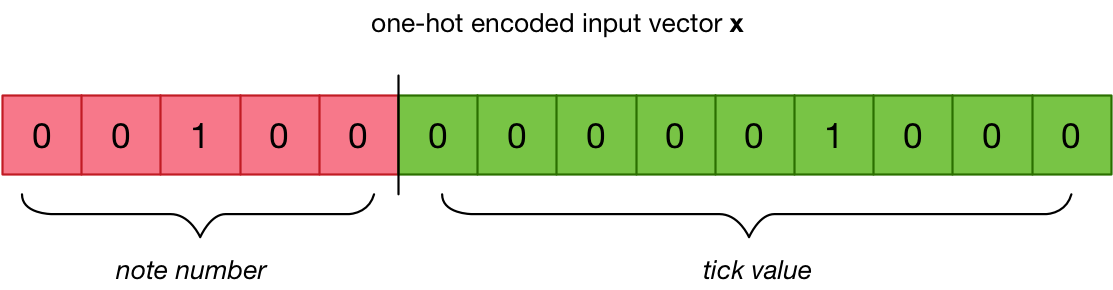
In the full dataset there are 17 unique note numbers and 209 unique tick values, so this vector consists of 226 elements. (Of those elements, 224 are 0 and two are 1.)

The sequence that we present to the RNN does not really exist of (note, ticks) pairs but is a list of these one-hot encoded vectors:

[ 0, 0, 1, 0, 0, 0, ..., 0 ] 
[ 1, 0, 0, 0, 0, 0, ..., 0 ] 
[ 0, 0, 0, 1, 0, 0, ..., 1 ]
. . . and so on . . .

Because there are 52260 notes in the dataset, the entire training sequence is made up of 52260 of those 226-element vectors.

The script convert_midi.py reads the MIDI files from the dataset and outputs a new file X.npy that contains this 52260×226 matrix with the full training sequence. (The script also saves two lookup tables that tell us which note numbers and tick values correspond to the positions in the one-hot vectors.)

Long Short-Term Memory (huh?!)

The kind of recurrent neural network we’re using is something called an LSTM or Long Short-Term Memory. It looks like this on the inside:

The vector x is a single input that we feed into the network. It’s one of those 226-element vectors from the training sequence that combines the note number and the delay in ticks for a single drum sound.

The output y is the prediction that is computed by the LSTM. This is also a 226-element vector but this time it contains a probability distribution over the possible note numbers and tick values. The goal of training the LSTM is to get an output y that is (mostly) equal to the next element from the training sequence.

Recall that a recurrent network has “internal state” that acts as its memory. The internal state of the LSTM is given by two vectors: c and h. The c vector helps the LSTM to remember the sequence of MIDI notes it has seen so far, and h is used to predict the next notes in the sequence.

At every time step we compute new values for c and h, and then feed these back into the network so they are used as inputs for the next timestep.

The most interesting feature of the LSTM is that it has gates that can be either 0 (closed) or 1 (open). The gates determine how data flows through the LSTM layer.

The gates perform different jobs:

• The “input” gate i determines whether the input x is added to the memory vector c. If this gate is closed, the input is basically ignored.
• The g gate determines how much of input x gets added to c if the input gate is open.
• The “output” gate o determines what gets put into the new value of h.
• The “forget” gate f is used to reset parts of the memory c.

The inputs x and h are connected to these gates using weights — Wxf, Whf, etc. When we train the LSTM, what it learns are the values of those weights. (It does not learn the values of h or c.)

Thanks to this mechanism with the gates, the LSTM can remember things over the long term, and it can even choose to forget things it no longer considers important.

Confused how this works? It doesn’t matter. Exactly how or why these gates work the way they do isn’t very important for this blog post. (If you really want to know, read the paper.) Just know this particular scheme has proven to work very well for remembering long sequences.

Our job is to make the network learn the optimal values for the weights between x and h and these gates, and for the weights between h and y.

The math

To implement an LSTM any sane person would use a tool such as Keras which lets you simply write layer = LSTM(). However, we are going to do it the hard way, using primitive TensorFlow operations.

The reason for doing it the hard way, is that we’re going to have to implement this math ourselves in the iOS app, so it’s useful to understand the formulas that are being used.

The formulas needed to implement the inner logic of the LSTM layer look like this:

f = tf.sigmoid(tf.matmul(x[t], Wxf) + tf.matmul(h[t - 1], Whf) + bf)
i = tf.sigmoid(tf.matmul(x[t], Wxi) + tf.matmul(h[t - 1], Whi) + bi)
o = tf.sigmoid(tf.matmul(x[t], Wxo) + tf.matmul(h[t - 1], Who) + bo)
g =    tf.tanh(tf.matmul(x[t], Wxg) + tf.matmul(h[t - 1], Whg) + bg)

What goes on here is less intimidating than it first appears. Let’s look at the line for the f gate in detail:

f = tf.sigmoid(
                 tf.matmul(x[t], Wxf)         # 1
               + tf.matmul(h[t - 1], Whf)     # 2
               + bf                           # 3
              )

This computes whether the f gate is open (1) or closed (0). Step-by-step this is what it does:

1. First multiply the input x for the current timestep with the matrix Wxf. This matrix contains the weights of the connections between x and f.

2. Also multiply the input h with the weights matrix Whf. In these formulas, t is the index of the timestep. Because h feeds back into the network we use the value of h from the previous timestep, given by h[t - 1].

3. Add a bias value bf.

4. Finally, take the logistic sigmoid of the whole thing. The sigmoid function returns 0, 1, or a value in between.

The same thing happens for the other gates, except that for g we use a hyperbolic tangent function to get a number between -1 and +1 (instead of 0 and 1). Each gate has its own set of weight matrices and bias values.

Once we know which gates are open and which are closed, we can compute the new values of the internal state c and h:

c[t] = f * c[t - 1] + i * g
h[t] = o * tf.tanh(c[t])

We put the new values of c and h into c[t] and h[t], so that these will be used as the inputs for the next timestep.

Now that we know the new value for the state vector h, we can use this to predict the output y for this timestep:

y = tf.matmul(h[t], Why) + by

This prediction performs yet another matrix multiplication, this time using the weights Why between h and y. (This is a simple affine function like the one that happens in a fully-connected layer.)

Recall that our input x is a vector with 226 elements that contains two separate data items: the MIDI note number and the delay in ticks. This means we also need to predict the note and tick values separately, and so we use two softmax functions, each on a separate portion of the y vector:

y_note[t] = tf.nn.softmax(y[:num_midi_notes])
y_tick[t] = tf.nn.softmax(y[num_midi_notes:])

And that’s in a nutshell how the math in the LSTM layer works. To read more about these formulas, see the Wikipedia page.

Too many matrices!

As you know, when a neural network is trained it will learn values for the weights and biases. The same is true here: the LSTM will learn the values of Wxf, Whf, bf, Why, by, and so on. Notice that this is 9 different matrices and 5 different bias values.

We can be clever and actually combine these matrices into one big matrix:

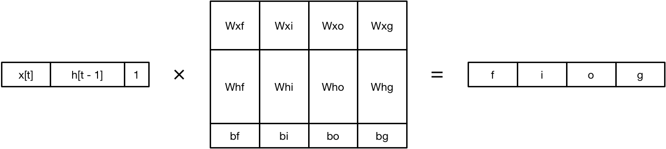
We first put the value of x for this timestep and the value of h of the previous timestep into a new vector (plus the constant 1, which gets multiplied with the bias). Likewise, we put all the weights and biases into one matrix. And then we multiply these two together.

This does the exact same thing as the eight matrix multiplies from before. The big advantage is that we now have to manage only a single weight matrix for x and h (and no bias value, since that is part of this big matrix too).

We can simplify the computation for the gates to just this:

combined = tf.concat([x[t], h[t - 1], tf.ones(1)], axis=0)
gates = tf.matmul(combined, Wx)

And then compute the new values of c and h as follows:

c[t] = tf.sigmoid(gates[0])*c[t - 1] + tf.sigmoid(gates[1])*tf.tanh(gates[3])
h[t] = tf.sigmoid(gates[2])*tf.tanh(c[t])

These two formulas for c and h didn’t really change — I just moved the sigmoid and tanh functions here.

Now when we train the LSTM we only have to deal with two weight matrices: Wx, which is the big matrix I showed you here, and Wy, the matrix that for the weights between h and y. Those two matrices are the learned parameters that get loaded into the iOS app.

Training

OK, let’s recap where we are now:

• We’ve got a dataset of 52260 one-hot encoded vectors that describe MIDI notes and their timing. Together, these 52260 vectors make up a very long sequence of drum patterns.

• We want to train the LSTM to memorize this sequence. In other words, for every note of the sequence the LSTM should be able to correctly predict the note that follows.

• We have the formulas for computing what happens in an LSTM layer. It takes an input x, which is one of these vectors describing a single drum sound, and two state vectors h and c. The LSTM then computes new values for h and c, as well as a prediction y for what the next note in the sequence will be.

Now we need to put this all together to train the recurrent network. This will give us two matrices Wx and Wy that describe the weights of the connections between the different parts of the LSTM.

And then we can use those weights in the iOS app to play new drum patterns.

A few notes about training

Training an LSTM isn’t very different from training any other neural network. We use backpropagation with an SGD (Stochastic Gradient Descent) optimizer and we train until the loss is low enough.

However, the nature of this network being recurrent — where the outputs h and c are always connected to the inputs h and c — makes backpropagation a little tricky. We don’t want to get stuck in an infinite loop!

The way to deal with this is a technique called backpropagation through time where we backpropagate through all the steps of the entire training sequence.

In the interest of keeping this blog post short, I’m not going to explain the entire training procedure here. You can find the complete implementation in lstm.py in the function train().

However, I do want to mention a few things:

• The learning capacity of the LSTM is determined by the size of the h and c vectors. A size of 200 units (or neurons if you will) seems to work well. More units might work even better but at some point you’ll get diminishing returns, and you’re better off stacking multiple LSTMs on top of each other (making the network deeper rather than wider).

• It’s not practical to backpropagate through all 52260 steps of the training sequence, even though that would give the best results. Instead, we only go back 200 timesteps. After a bit of experimentation this seemed like a reasonable number. To achieve this, the training script actually sticks 200 LSTM units together and processes the training sequence in chunks of 200 notes at a time.

• Every so often the training script computes the percentage of predictions it has correct. It does this on the training set (there is no validation set) so take it with a grain of salt, but it’s a good indicator of whether the training is still making progress or not.

• The final model took a few hours to train on my iMac but that’s because it doesn’t have a GPU that TensorFlow can use (sad face). I let the training script run until the learning seemed to have stalled (the accuracy and loss did not improve), then I pressed Ctrl+C, lowered the learning rate in the script, and resumed training from the last checkpoint.

The model that is included in the GitHub repo has an accuracy score of about 92%, which means 8 in every 100 notes from the training sequence are remembered wrong. Once the model reached 92% accuracy, it didn’t seem to want to go much further than that, so we’ve probably reached the capacity of our model.

An accuracy of “only” 92% is good enough for our purposes: we don’t want the LSTM to literally remember every example from the training data, just enough to get a sense of what it means to play the drums.

So how good is it?

Don’t fire the drummer from your band just yet. :–)

The question is: has the recurrent neural network really learned anything from the training data, or does it just output random notes?

Here’s an MP3 of randomly chosen notes and durations from the training data. It doesn’t sound like real drums at all.

Compare it with this recording that was produced by the LSTM. It’s definitely much more realistic! (In fact, it sounds a lot like the kid down the street practicing.)

Of course, the model we’re using is very basic. It’s a single LSTM layer with “only” 200 neurons. No doubt there are much better ways to train a computer to play the drums. One way is to make the network deeper by stacking multiple LSTMs. This should improve the performance by a lot!

The weights that are learned by the model take up 1.5 MB of storage. The dataset, on the other hand, is only 1.3 MB! That doesn’t seem very efficient. But just having the dataset does not mean you know how to drum — the weights are more than just a way to remember the training data, they also “understand” in some way what it means to play the drums.

The cool thing is that our neural network doesn’t really know anything about music: we just gave it examples and it has learned drumming from that (to some extent anyway). The point I’m trying to make with this blog post is that if we can make a recurrent neural network learn to drum, then we can teach it to understand any kind of sequential data.

The iOS app

Finally we get to the Swift portion of this blog post!

The iOS app is very simple: it just has a button. When you tap the button, the app generates a new drum sequence of 1,000 notes and plays it using AVMIDIPlayer.

The interesting part of the app is in how it generates the drum sequence. The code uses the same LSTM math as above, except this time it’s not implemented using TensorFlow but with functions from the Accelerate framework.

In pseudocode the algorithm looks like this:

randomize the c and h vectors
choose a random starting note and ticks

repeat 1000 times:
    one-hot encode the note/ticks pair
    do the LSTM math
    add the predicted next note and duration to an array
    use this new note/ticks pair as the new input  

Each iteration of the loop predicts a new note and duration, then uses this to predict another note and duration, and so on. This gives us an array of 1,000 (note, ticks) pairs.

The full code is in Drummer.swift in the function sample(). I’m not going to show every single step, but here are a few snippets.

First, we start with random c and h vectors. Recall that these make up the internal state of the LSTM. During training this internal state kept track of where we were in the training sequence. But now we want to create original drum patterns, so we start off with a randomized memory state.

Math.uniformRandom(&c, hiddenSize, 0.1)
Math.uniformRandom(&h, hiddenSize, 0.1)

The Math namespace is an enum that contains static functions that wrap around the Accelerate functionality. It makes the Accelerate framework a little easier to use. (See Math.swift for details.)

uniformRandom() fills up the c and h arrays with random floating-point values between -0.1 and +0.1. Feel free to experiment and make these values larger or smaller to get different prediction results.

Inside the loop, we first one-hot encode the current note number and ticks value. As before, we put these into a 226-element vector. We also append h to this vector and add a 1 at the end. As you’ve seen above, this allows us to do all of the LSTM weight calculations with a single matrix.

The code for doing the matrix multiply is:

Wx_data.withUnsafeBytes { Wx in
  Math.matmul(&x, Wx, &gates, 1, Wx_cols, Wx_rows)
}

where Wx_data is a Data object with the contents of the file Wx.bin. We multiply x, which is the vector containing the one-hot note and ticks as well as h, with the big weight matrix Wx and we store the result in the new array gates.

Let’s take a look at Math.matmul() to see what it does:

enum Math {
  static func matmul(_ A: UnsafePointer<Float>, 
                     _ B: UnsafePointer<Float>, 
                     _ C: UnsafeMutablePointer<Float>, 
                     _ M: Int, _ N: Int, _ K: Int) {
    cblas_sgemm(CblasRowMajor, CblasNoTrans, CblasNoTrans, 
                Int32(M), Int32(N), Int32(K), 1, A, 
                Int32(K), B, Int32(N), 0, C, Int32(N))
  }
}

This is just a simple wrapper around the cblas_sgemm() function, which multiplies matrix (or vector) A with matrix B and stores the result in matrix C. (M, N, and K are the dimensions of the matrices.)

Most of the other Math functions are simple one-liners too, but some — such as sigmoid() and softmax() — are more complicated, as their calculations need to combine multiple Accelerate functions.

The next bit performs the LSTM math:

gates.withUnsafeMutableBufferPointer { ptr in
  let gateF = ptr.baseAddress!
  let gateI = gateF.advanced(by: hiddenSize)
  let gateO = gateI.advanced(by: hiddenSize)
  let gateG = gateO.advanced(by: hiddenSize)

  // Compute the activations of the gates.
  Math.sigmoid(gateF, hiddenSize*3)
  Math.tanh(gateG, hiddenSize)

  // c[t] = sigmoid(gateF) * sigmoid(c[t-1]) + sigmoid(gateI) * tanh(gateG)
  Math.multiply(&c, gateF, &c, hiddenSize)
  Math.multiply(gateI, gateG, &tmp, hiddenSize)
  Math.add(&tmp, &c, hiddenSize)

  // h[t] = sigmoid(gateO) * tanh(c[t])
  Math.tanh(&c, &tmp, hiddenSize)
  Math.multiply(gateO, &tmp, &h, hiddenSize)
}

In the Python code we could do this in just three lines but in Swift it’s a bit more verbose. At the end of this block of code we have the new values for the internal state vectors c and h.

Now that we know h, we can compute the prediction y:

Wy_data.withUnsafeBytes { Wy in
  Math.matmul(&h, Wy, &y, 1, Wy_cols, Wy_rows)
}

y.withUnsafeMutableBufferPointer { ptr in
  let yNote = ptr.baseAddress!
  let yTick = yNote.advanced(by: noteVectorSize)

  Math.softmax(yNote, noteVectorSize)
  Math.softmax(yTick, tickVectorSize)

As before, we first multiply h by the weight matrix Wy to get the 226-element vector y. Then we take the softmax twice, once to predict the next note number and once to predict the next duration in ticks.

The softmax gives us two probability distributions: one for the note numbers and one for the ticks. What we do with those probability distributions is slightly different than in the training procedure:

  let noteIndex = Math.randomlySample(yNote, noteVectorSize)
  let tickIndex = Math.randomlySample(yTick, tickVectorSize)
  sampled.append((index2note[noteIndex], index2tick[tickIndex]))

The randomlySample() function picks a value based on the probabilities. Suppose you have an array of probabilities [ 0.2, 0.8 ] and you run randomlySample() on that array 100 times, it will pick the first element about 20 times and the second element about 80 times.

So here we choose one value from each probability distribution — the higher its probability the more likely we’ll choose it — and those are the note and ticks we’ll use for this timestep.

Now that we’ve predicted a new note and duration, we feed the new c and h vectors back into the network and repeat the loop. And that’s all we need to do to generate a new drum sequence! We simply run the LSTM math 1,000 times in a row.

To actually play the drums through the iPhone’s speaker, the app turns the array of predicted (note, ticks) pairs into a MusicSequence object and then gives that to AVMIDIPlayer. For the exact details, check out ViewController.swift.

Give it a try! Download the GitHub repo and build the Drummer.xcodeproj file with Xcode 8. Be sure to run the app on a device because MIDI playback on the simulator is broken. And remember that each time you tap the button, the drummer starts with a random memory, so sometimes the results will be better than others. 😅

Credits

The RNN training procedure is based on the min-char-rnn.py code sample from Andrej Karpathy. See also his excellent blog post “The Unreasonable Effectiveness of Recurrent Neural Networks”.

The iOS code for MIDI playback was based on this blog post by Gene De Lisa.

The SoundFont used in the iOS app was downloaded here.