The lost art of 3D rendering without shaders

Let’s say you wanted to create a sweet bouncing cube, like this:

You might use a 3D framework such as OpenGL or Metal. That involves writing one or more vertex shaders to transform your 3D objects, and one or more fragment shaders to draw these transformed objects on the screen.

The framework then takes these shaders and your 3D data, performs some magic, and paints everything in glorious 32-bit color.

But what exactly is that magic that OpenGL and Metal do behind the scenes?

Back in the day — way before we had hardware accelerated 3D graphics cards, let alone programmable GPUs — if you wanted to draw a 3D scene you had to do all that work yourself. In assembly. On a computer with a 7 MHz processor.

I’ve got a shelf full of books on 3D graphics that are obsolete because nowadays you can simply use OpenGL or Metal. And I’m glad we can! However, even if you take advantage of these modern GPUs and 3D APIs, it’s still useful to understand the steps that are involved in drawing 3D objects on the screen.

In this post I’ll explain how to draw a 3D bouncing cube, with simple animation and lighting, but without using shaders. It illustrates what happens under the hood when you use OpenGL or Metal, and I’ll point out where the modern vertex and fragment shaders fit into this story.

We won’t use any 3D APIs at all — this is as basic as it gets. The only rendering primitive we have at our disposal is a setPixel() function to write individual pixels into a 800×600 bitmap:

func setPixel(x: Int, y: Int, r: Float, g: Float, b: Float, a: Float)

This changes the pixel at bitmap coordinates (x, y) to the color (r, g, b, a). Everything else we need to do in order to draw in 3D is built on top of this very basic setPixel() function, and is explained below in detail.

After reading this post you will be able to write your own basic 3D renderer from scratch and understand a bit better how the OpenGL and Metal pipelines work.

The demo app

If you want to have a look at the finished app, you can find the full source code on GitHub. This is a macOS app, written in Swift 3. (The language isn’t really important, you can easily port this to any other language.)

Just open the project in Xcode 8 and run it. The demo shows a colored cube that bounces up and down and spins around the vertical axis:

The slider at the top moves the camera left or right, to let you look at the cube from different vantage points.

The app isn’t particularly pretty but it does demonstrate many of the concepts involved in 3D rendering.

All the important code is in the file Render.swift. It has lots of explanations, so you could just read the source instead of this blog post. 😉

In short, what happens in the demo app is this: the function render() takes some 3D model data (the cube), transforms and projects it, and then draws it by calling setPixel() over and over (which is why it is so slow).

What happens in render() is roughly what happens on the GPU when you tell OpenGL or Metal to draw 3D stuff on the screen. But instead of using shaders, we’re doing it all by hand.

Let’s take a look at all the pieces you need to make this happen.

The 3D model

First we define the model. This is the 3D object that we want to draw. The model is made up of triangles because triangles are easy to draw. These triangles are also called the geometry of the model.

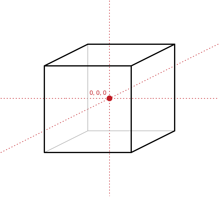
The geometry for the cube looks like this:

As you can see, the size of this cube goes from -10 units to +10 units. The units can be whatever you want, so let’s say centimeters.

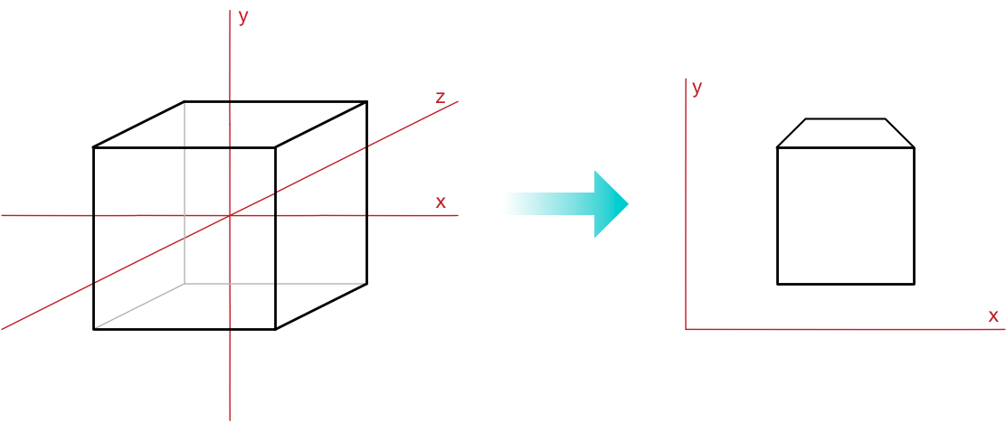
The coordinate system we use looks like this:

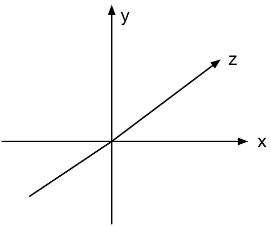
The x-coordinate is positive to the right, y is postive going up, and z is positive going into the screen. This is a so-called left-handed coordinate system.

Each triangle consists of 3 vertices. A vertex describes an (x, y, z) position in 3D space, but also the color of the triangle at that vertex and a normal vector for lighting calculations. You can also add extra information such as texture mapping coordinates, as well as any other data you want to associate with a vertex.

struct Vertex {
  var x: Float = 0   // coordinate in 3D space
  var y: Float = 0
  var z: Float = 0

  var r: Float = 0   // color
  var g: Float = 0
  var b: Float = 0
  var a: Float = 1

  var nx: Float = 0  // normal vector (using for lighting)
  var ny: Float = 0
  var nz: Float = 0
}

struct Triangle {
  var vertices = [Vertex](repeating: Vertex(), count: 3)
}

To implement the 3D model for the cube, then, we just need to provide a list of these triangles. You would typically design your model in a tool like Blender and load it from a .obj file but because this is a simple demo we define the geometry by hand:

let model: [Triangle] = {
  var triangles = [Triangle]()

  // The first triangle
  var triangle = Triangle()
  triangle.vertices[0] = Vertex(x: -10, y: -10, z: 10,    // position
                                r: 0, g: 0, b: 1, a: 1,   // color 
                                nx: 0, ny: 0, nz: 1)      // normal
  triangle.vertices[1] = Vertex(x: -10, y: 10, z: 10, 
                                r: 0, g: 0, b: 1, a: 1,
                                nx: 0, ny: 0, nz: 1)
  triangle.vertices[2] = Vertex(x: 10, y: -10, z: 10, 
                                r: 0, g: 0, b: 1, a: 1,
                                nx: 0, ny: 0, nz: 1)
  triangles.append(triangle)

  // The second triangle
  triangle = Triangle()
  triangle.vertices[0] = Vertex(x: -10, y: 10, z: 10, 
                                r: 0, g: 0, b: 1, a: 1,
                                nx: 0, ny: 0, nz: 1)
  triangle.vertices[1] = // . . . and so on . . . 

  return triangles
}()

There are 12 triangles in this model, so 36 vertices in total. Each vertex has its own position (x, y, z), color (r, g, b, a), and normal vector (nx, ny, nz).

The normal vector should have length 1 and point away from the triangle. This determines which direction that triangle faces, something we need to calculate the influence of any lights.

Note that some of the x, y, z-coordinates are at -10 and some are at +10. This is done so that the center of the cube is at the origin (0, 0, 0). This is called the local origin of the model. (We need this local origin so that we can rotate the object around its center.)

Even if we want the cube to be somewhere else in the 3D world instead of on the origin, we still design the model so that its center is at (0, 0, 0). Then later on, we’ll move the cube to its final position in the world. That’s what happens in the next section.

Where does the model live in the world?

The cube not only has vertices and triangles that determine its shape, but it also has a position in the 3D world, a scale, and an orientation that is given by three rotation angles (also known as pitch, roll, and yaw). We define variables for these properties:

var modelX: Float = 0
var modelY: Float = 0
var modelZ: Float = 0

var modelScaleX: Float = 1
var modelScaleY: Float = 1
var modelScaleZ: Float = 1

var modelRotateX: Float = 0
var modelRotateY: Float = 0
var modelRotateZ: Float = 0

Initially, we place the model at the center of our world at coordinates (0, 0, 0), give it a scale of 1 (or 100%) in each direction, and set all rotation angles to zero.

There is some code in ViewController.swift that performs animations. It has a timer that fires every few milliseconds. In the timer method, we make changes to the above variables, which makes the cube move through the 3D world, and then we call render() to redraw the entire 3D scene to show these changes.

For example, to make the cube bounce, we change the modelY variable so that the cube moves up and down. When the cube hits the floor it gets “flattened” a little by changing modelScaleX/Y/Z. And the cube appears to spin because at every animation step we increment modelRotateY.

Remember that the model has a so-called “local” origin? This tells you where the center of the model is. There is a conceptual difference between the center of the world and the center of the model, even though both have coordinates (0, 0, 0). Any movement of the model through the world is relative to that local origin.

For the cube as we’ve currently defined it, its local origin is at the exact center of the cube. However, if you load a model from a .obj file the local center may not be exactly where you want it to be. We can fix this by declaring where the local origin of the model should be, relative to the positions of its vertices:

var modelOriginX: Float = 10
var modelOriginY: Float = 0
var modelOriginZ: Float = 10

Note that we did not use (0, 0, 0) here, but (10, 0, 10), which is one of the corners of the cube. Rotations happen around this local origin, and just for the fun of it the demo app will be rotating around one of the corners instead of the center.

If you’re running the demo app, feel free to play with any of these variables and the animation code to see what happens. It’s fun!

The camera

So far we’ve defined a 3D object and have given it a place in our 3D world. The cube currently sits at the center of the world and we can move it by changing the model* variables. (That’s how we’re making it bounce up and down.)

But where do you, the observer, sit in the world? Currently, you also sit at the origin, i.e. smack in the middle of the cube. If we were to render the 3D scene now, you’d see the cube from the inside out.

We can introduce a camera object, which also has a position in the 3D world. This object does not have any geometry, but it simply represents where the observer is in the world and where it is looking.

var cameraX: Float = 0
var cameraY: Float = 20
var cameraZ: Float = -20

In the demo app, I’ve moved the camera up by 20 units, so you’re looking slightly down at the scene (you can see the top of the cube but not its bottom).

The camera is also pulled backwards by -20 units along the Z-axis, making it appear as if the cube is moved away from the observer and into the screen. In other words, we’ll be looking at the cube from a “safe” distance.

When you drag the slider in the app, you change cameraX.

The lights

When we defined the 3D geometry for the cube, we gave each vertex a color. We could simply draw the triangles using the colors of their vertices but that’s a little bland. To make 3D scenes look more interesting we want to have realistic lighting effects.

The following options control the lighting of the scene. First, there is ambient light, this is “background” light that’s always there:

var ambientR: Float = 1
var ambientG: Float = 1
var ambientB: Float = 1
var ambientIntensity: Float = 0.2

The ambient light we’ve defined here is pure white but only has 20% intensity. This means when we apply this light, we multiply the vertex colors by (0.2, 0.2, 0.2), making them a lot darker. (That’s OK because we’ll also apply directional lighting to make them brighter again.)

You can play with these ambient settings to give the entire scene a certain feel. If you were to set ambientB = 0, for example, then all vertices would only keep their red + green components and all blue light would get filtered out.

If you set ambientIntensity to 0.0, then in absense of any other light sources, the cube will be completely black. If set to 1.0, the ambient light drowns out any other light sources.

We also define a diffuse light source. Like ambient light, this has a color and an intensity, but also a direction:

var diffuseR: Float = 1
var diffuseG: Float = 1
var diffuseB: Float = 1
var diffuseIntensity: Float = 0.8

var diffuseX: Float = 0    // direction of the diffuse light
var diffuseY: Float = 0    // (this vector should have length 1)
var diffuseZ: Float = 1

For our demo app, the diffuse light source is pointing into the positive z-direction, which means there is a light source shining in the same direction as the camera is looking. The more a side of the cube is aligned with the camera — and therefore the light source — the brighter it will appear.

In the image below on the left, the cube’s green side is facing the directional light and therefore it shows up as bright green. But as the cube rotates away from the light, the green side becomes darker (and the blue side becomes brighter):

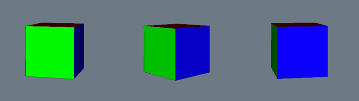
There is no light source shining on the cube from above, so the red triangles at the top will look quite dark as they are only illuminated by the ambient light.

Action!

OK, so far we’ve just defined the data structures and variables that our 3D scene will use. Now it’s time to show how to actually render this 3D world on the screen.

The function render() is called on every animation frame. This function takes the model’s vertex data, its state (modelX, modelRotateY, etc), and the position of the camera, and produces a 2D rendition of the 3D scene.

In a real game, render() would ideally be called 60 times per second (or more). With OpenGL or Metal, calling render() would be equivalent to setting up your shaders and then calling glDrawElements() or MTLCommandBuffer.commit().

Here is the rendering pipeline that is performed by render():

I’ll explain in detail what happens in each of these steps.

The code for render() itself is quite simple, as it farms out most of the work to helper functions. Here is the code:

func render() {
  // 1: Erase what we drew last time.
  clearRenderBuffer(color: 0xff302010)

  // 2: Also clear out the depth buffer.
  for i in 0..<depthBuffer.count {
    depthBuffer[i] = Float.infinity
  }

  // 3: Take the cube, place it in the 3D world, adjust the viewpoint for
  // the camera, and project everything to two-dimensional triangles.
  let projected = transformAndProject()

  // 4: Draw these 2D triangles on the screen.
  for triangle in projected {
    draw(triangle: triangle)
  }
}

First, it removes everything that it drew in the previous frame so that we can start with a clear slate. (Step 1 and 2)

Then it calls transformAndProject() to convert the 3D cube into a list of two-dimensional triangles. This is roughly equivalent to what happens in a vertex shader. (Step 3)

Finally, it calls draw(triangle) to render each of these 2D triangles on the screen. This is what happens in a fragment shader. For example, the calculations to apply the lighting are done here. (Step 4)

I haven’t mentioned the depth buffer from step 2 yet. This is used to make sure far away triangles don’t overlap closer triangles. The depth buffer is defined as:

var depthBuffer: [Float] = {
  return [Float](repeating: 0, count: Int(context!.width * context!.height))
}()

where context!.width and .height are the size of the screen. In the demo app it is 800×600 pixels, the same size as the render buffer. To clear out the depth buffer, we will it with large values, Float.infinity. I’ll have more to say about how this depth buffer works later.

Let’s look at the helper function from step 3 now, transformAndProject().

Transforming the triangles

This concerns the first three actions in the flow chart.

Each 3D model in the app (we only have one, the cube) is defined in its own, local coordinate space (aka model space). In order to draw these models on the screen, we have to make them undergo several “transformations”:

1. First we have to place the model inside the 3D world. This is a transformation from model space to world space. Theoretically you could define the cube in world space coordinates already, but it’s easier to create the model inside its own tiny universe, independent of any other models, and then place it into the larger world by translating, scaling, and rotating it.

2. Then we position the camera and look at the world through this camera, a transformation from world space to camera space (or “eye space”). At this point we can already throw away some triangles that are not visible because they are facing away from the camera or because they are behind the camera.

3. Finally, we project the 3D view from the camera onto a 2D surface so that we can show it on the screen; this projection is a transformation to screen space (also known as “viewport space”).

These transformations is where all the math happens. To make clear what is going on, I will use only straightforward math — mostly addition, multiplication, and the occasional sine and cosine.

A lot of the stuff that happens in transformAndProject() would normally be done by a vertex shader on the GPU. The vertex shader takes the model’s vertices and transforms them from local 3D space to 2D space, and all the steps inbetween.

We will now look at each of these transformations in detail.

Model space to world space

Inside the transformAndProject() function, we first perform the transformation to world space.

We want the cube to spin around and bounce up and down. So we take the original vertices that define the cube’s geometry (which are centered around the cube’s local origin) and move them from this local model space into the larger world.

For this transformation we’ll use the modelXYZ, modelRotateXYZ, modelScaleXYZ variables we defined earlier (recall these are the variables that get changed by the animation code).

The transformation happens in a loop because we need to apply it to each of the model’s vertices in turn. We store the results in a new (temporary) array because we don’t want to overwrite the original cube data. The loop looks like this:

var transformed = model

// Look at each triangle...
for (j, triangle) in transformed.enumerated() {
  var newTriangle = Triangle()

  // Look at each vertex of the triangle...
  for (i, vertex) in triangle.vertices.enumerated() {
    var newVertex = vertex

    // TODO: the math happens here

    // Store the new vertex into the new triangle.
    newTriangle.vertices[i] = newVertex
  }
  
  // Store the new triangle into the model.
  transformed[j] = newTriangle
}

To not overwhelm you with a massive wall of code, I left out the code for the different transformation steps. We’ll now look at these steps one-by-one. Just remember we apply this math to all of the vertices from the 3D model.

The local origin

First, we may need to adjust the model’s origin, which is a translation (math speak for “movement”). If modelOriginX, Y, or Z are not (0, 0, 0), then we want (modelOriginX, modelOriginY, modelOriginZ) to become the new center of the model. We do that by subtracting these values from the coordinates of the vertex:

newVertex.x -= modelOriginX
newVertex.y -= modelOriginY
newVertex.z -= modelOriginZ

Since the coordinate of the vertex is relative to the model’s local origin, to adjust this local origin we need to move the vertex — but in the opposite direction.

Scaling

Next, we’ll apply scaling (if any). Scaling is useful if you’re loading a model from a .obj file and it doesn’t use the same units as your 3D world (meters vs centimeters, for example), but it’s also great for special effects. In this demo we’re using scaling to exaggerate the “bouncing” motion.

Scaling is a simple multiplication:

newVertex.x *= modelScaleX
newVertex.y *= modelScaleY
newVertex.z *= modelScaleZ

By default modelScaleX, Y, and Z are all 1, so the multiplication has no effect. But if the scaling factor is greater than 1, the vertex will move further away from the model’s local origin, making the model appear bigger; for a scaling factor smaller than 1, the vertex will move closer to the origin.

Rotations

Next up are the rotations. This uses a bit of trigonometry but you don’t need to memorize these formulas. (I keep them on a cheatsheet.)

First, we rotate about the X-axis, then about the Y-axis, and finally about the Z-axis.

The order in which you perform these rotations doesn’t really matter, although there is an issue called gimbal lock that you need to be aware of. It basically means that if you combine certain rotations that you lose track of where you are heading. (One solution to this is to use more fancy math.)

// Rotate about the X-axis.
var tempA =  cos(modelRotateX)*newVertex.y + sin(modelRotateX)*newVertex.z
var tempB = -sin(modelRotateX)*newVertex.y + cos(modelRotateX)*newVertex.z
newVertex.y = tempA
newVertex.z = tempB

// Rotate about the Y-axis:
tempA =  cos(modelRotateY)*newVertex.x + sin(modelRotateY)*newVertex.z
tempB = -sin(modelRotateY)*newVertex.x + cos(modelRotateY)*newVertex.z
newVertex.x = tempA
newVertex.z = tempB

// Rotate about the Z-axis:
tempA =  cos(modelRotateZ)*newVertex.x + sin(modelRotateZ)*newVertex.y
tempB = -sin(modelRotateZ)*newVertex.x + cos(modelRotateZ)*newVertex.y
newVertex.x = tempA
newVertex.y = tempB

These formulas rotate the vertex around the model’s adjusted origin. This is why it’s important to make a distinction between the center of the model and the center of the world, because you don’t want the vertex to rotate around the center of the entire world.

The normal vector

Recall that the vertex doesn’t just have a coordinate in 3D space, it also has a normal vector. This normal vector describes the direction the vertex (or its triangle) is pointing in. We need to rotate the normal vector so that it stays aligned with the orientation of the vertex. Because in this demo app we only rotate about the Y-axis, I’ve only included that rotation formula, and not for the other axes.

tempA =  cos(modelRotateY)*newVertex.nx + sin(modelRotateY)*newVertex.nz
tempB = -sin(modelRotateY)*newVertex.nx + cos(modelRotateY)*newVertex.nz
newVertex.nx = tempA
newVertex.nz = tempB

Translation

Finally, perform translation to the model’s destination location in the 3D world:

newVertex.x += modelX
newVertex.y += modelY
newVertex.z += modelZ

OK, that completes the translations used to position and orient the 3D model in the 3D world. Now the model is scaled, rotated, and put in its proper place.

As you can see, we’re doing quite a few calculations to get the model from its local coordinate system into world space, and we need to perform them for every single vertex in our model. And if we had multiple models, as most games tend to do, we’d need to repeat all these calculations for each model.

That’s why in practice you’d put these calculations into a matrix and then you just have to multiply each vertex with that matrix. That’s much simpler and more efficient because it can be hardware accelerated — either on the CPU by simd instructions or on the GPU by the vertex shader. It’s common to compute the matrix on the CPU, then pass it to the vertex shader, which will use it to transform all the vertices.

World space to camera space

Currently we’re viewing the 3D world from (0, 0, 0), straight down the z-axis. But in a real 3D app, the observer may not always be in a fixed position.

You can imagine we’re viewing the world through a “camera” object, and we can place this camera anywhere we want and make it look anywhere we want.

This means we need to transform the objects from “world space” into “camera space”. This uses the same math as before, but in the opposite direction.

  for (j, triangle) in transformed.enumerated() {
    var newTriangle = Triangle()
    for (i, vertex) in triangle.vertices.enumerated() {
      var newVertex = vertex

      // Move everything in the world opposite to the camera, i.e. if the
      // camera moves to the left, everything else moves to the right.
      newVertex.x -= cameraX
      newVertex.y -= cameraY
      newVertex.z -= cameraZ

      // Likewise, you can perform rotations as well. If the camera rotates
      // to the left with angle alpha, everything else rotates away from the
      // camera to the right with angle -alpha. (I did not implement that in
      // this demo.)

      newTriangle.vertices[i] = newVertex
    }
    transformed[j] = newTriangle
  }

In practice, you’d also use a matrix for this camera transformation. (In fact, you can combine the model matrix and the camera matrix into a single matrix, sometimes called the modelview matrix.)

Backface culling

At this point all the triangles are in “camera space”, so you know what portion of the world will be visible through the camera’s lens.

To save precious processing time you will want to throw away triangles that aren’t going to be visible anyway, for example those that are behind the camera or those that are facing away from the camera.

Metal or OpenGL will automatically do this for you.

I didn’t implement it in the demo app as it involves a bit more math than I want to explain here, but a common technique is backface culling.

Backface culling works by computing the angle between the orientation of the camera and the direction the triangle is facing. This tells you if the triangle is pointing towards the camera (i.e. visible) or away from it (invisible). You simply delete triangles that are facing the wrong way so they won’t get processed any further.

You can also throw away any triangles that are outside the field of view of the camera, known as the viewing frustum. But since this is only a simple demo app, I did not implement this either.

Camera space to screen space (or going from 3D to 2D)

Now we have a set of triangles described in camera space, which is expressed in three dimensions. But our computer’s screen is two-dimensional. In math terms, we need to project our triangles from 3D to 2D somehow.

The units of camera space are whatever you want them to be (we chose centimeters) but we need to convert this to pixels.

Also, we need to decide where on the screen to place the camera space’s origin (we’ll put it in the center). And we have to project from 3D coordinates to 2D, which requires getting rid of the z-axis.

That all happens in this final transformation step.

As before, I’ll illustrate how to do this transformation with basic math operations. Typically you’d combine all these operations into a projection matrix and pass that to your vertex shader, so applying it to the vertices would happen on the GPU.

Again, we loop through all the triangles and all the vertices. For each vertex we do the following:

newVertex.x /= (newVertex.z + 100) * 0.01
newVertex.y /= (newVertex.z + 100) * 0.01

A simple way to do a 3D-to-2D projection is to divide both x and y by z. The larger z is, the smaller the result of this division. Which makes sense because objects that are further away should appear smaller. In a real 3D app, you’d use a projection matrix that is a bit more elaborate but this is the general idea.

We need to do two more things. First, we convert our world units (centimeters) to pixels. In this demo app, I wanted the camera viewport to take up about -40 to +40 of our world units (centimeters). We need to scale up the vertex’s x and y values; we use the same amount in both directions, so everything stays square:

newVertex.x *= Float(contextHeight)/80
newVertex.y *= Float(contextHeight)/80

At long last, we’re now working in pixels!

Finally, we want (0, 0) to be in the center of the screen. Initially it is at the bottom-right corner, so shift everything over by half the screen size (in pixels).

newVertex.x += Float(contextWidth/2)
newVertex.y += Float(contextHeight/2)

Note that these formulas change only newVertex.x and .y but not .z. That makes sense because the triangles we’ll draw on the screen are now two-dimensional. But we still want to keep this z-value around. We can use it for filling in the depth buffer, which lets us determine whether to overwrite any existing pixels when we attempt to draw the triangles.

This completes the transformations. Let’s finally do some drawing!

Triangle rasterization

OK, so far what we’ve done is put our 3D model into the world, adjusted for the camera’s viewpoint, and converted to 2D space.

What we have now is the same list of triangles, but their vertex coordinates now represent specific pixels on the screen (instead of points in some imaginary three-dimensional space).

We can draw these three pixels for every triangle but that only gives us the vertices, it does not fill in the entire triangle. To fill up the triangles we have to connect these vertex pixels somehow. This is called rasterizing.

Metal takes care of most of this for you. Once it has figured out which pixels belong to the triangle, the GPU will call the fragment shader for each of these pixels — and that lets you change how each individual pixel gets drawn.

Still, it’s useful to understand how rasterizing works under the hood, so that is what we’ll go over in this section.

We need to figure out which pixels make up each triangle and what color they get. This happens in draw(triangle). The render() function calls draw(triangle) for each triangle in screen space.

This is what the draw(triangle) function does:

func draw(triangle: Triangle) {
  // 1. Only draw the triangle if it is at least partially inside the viewport.
  guard partiallyInsideViewport(vertex: triangle.vertices[0])
     && partiallyInsideViewport(vertex: triangle.vertices[1])
     && partiallyInsideViewport(vertex: triangle.vertices[2]) else {
    return
  }

  // 2. Reset the spans so that we're starting with a clean slate.
  spans = .init(repeating: Span(), count: context!.height)
  firstSpanLine = Int.max
  lastSpanLine = -1

  // 3. Interpolate all the things!
  addEdge(from: triangle.vertices[0], to: triangle.vertices[1])
  addEdge(from: triangle.vertices[1], to: triangle.vertices[2])
  addEdge(from: triangle.vertices[2], to: triangle.vertices[0])

  // 4. Draw the horizontal strips.
  drawSpans()
}

Step 1: OpenGL or Metal will have already thrown away any triangles that are not visible. Still, some of the triangles may be only partially visible. These will be clipped against the boundaries of the screen. In this demo app we take a simpler approach and simply don’t draw pixels if they fall outside the visible region.

Step 2, 3, 4: What happens in the rest of draw(triangle) I will explain below. Just note that it requires these additional variables:

var spans = [Span]()
var firstSpanLine = 0
var lastSpanLine = 0

Interpolation

To rasterize a triangle, we’ll draw horizontal strips. For example, if the triangle has these vertices,

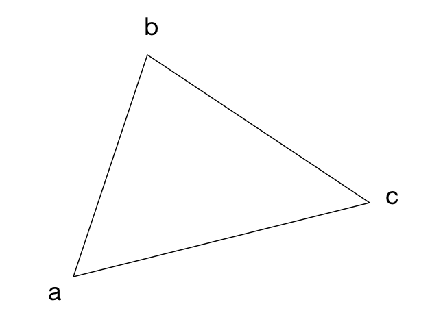
then the horizontal strips will look like this:

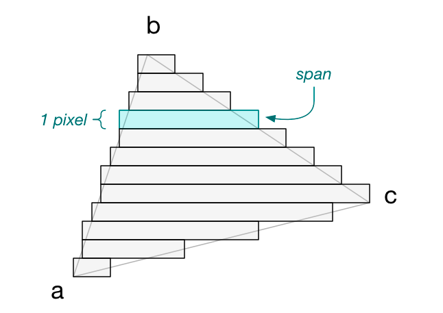
There is one strip for every vertical position on the screen, so strips are exactly 1 pixel high. I call these horizontal strips spans:

struct Span {
  var edges = [Edge]()

  var leftEdge: Edge {
    return edges[0].x < edges[1].x ? edges[0] : edges[1]
  }

  var rightEdge: Edge {
    return edges[0].x > edges[1].x ? edges[0] : edges[1]
  }
}

To find out where each span starts and ends, we have to start at vertex a and step vertically towards vertex b to find the corresponding x-positions on each line. We also do this from vertex a to c, and from c to b (always going up).

The points that we find I call edges:

An edge represents an x-coordinate. Each span has two edges, one on the left and one on the right. Once we’ve found these two edges, we simply draw a horizontal line between them. Repeat this for all the spans in the triangle, and we’ll have filled up the triangle with pixels!

struct Edge {
  var x = 0          // start or end coordinate of horizontal strip

  var r: Float = 0   // color at this point
  var g: Float = 0
  var b: Float = 0
  var a: Float = 0

  var z: Float = 0   // for checking and filling in the depth buffer

  var nx: Float = 0  // interpolated normal vector
  var ny: Float = 0
  var nz: Float = 0
}

The keyword in rasterization is interpolation. We interpolate all the things!

As we calculate these spans and their edges, we not only interpolate the x-positions of the vertices, but also their colors, their normal vectors, the z-values for the depth buffer, their texture coordinates, and so on.

For every single pixel in the triangle we will calculate an interpolated value for all of these properties.

The interpolation between the vertex properties happens in a helper function, addEdge(from:to:). Below is an abbreviated version of this function because there’s a bunch of duplicate code in there.

func addEdge(from vertex1: Vertex, to vertex2: Vertex) {
  let yDiff = ceil(vertex2.y - 0.5) - ceil(vertex1.y - 0.5)

  guard yDiff != 0 else { return }      // degenerate edge

  let (start, end) = yDiff > 0 ? (vertex1, vertex2) : (vertex2, vertex1)
  let len = abs(yDiff)

  var yPos = Int(ceil(start.y - 0.5))   // y should be integer because it
  let yEnd = Int(ceil(end.y - 0.5))     // needs to fit on a 1-pixel line

  let xStep = (end.x - start.x)/len     // x can stay floating point for now
  var xPos = start.x + xStep/2

  let rStep = (end.r - start.r)/len
  var rPos = start.r

  /* . . . more attributes here . . . */

  while yPos < yEnd {
    let x = Int(ceil(xPos - 0.5))       // now we make x an integer too

    // Don't want to go outside the visible area.
    if yPos >= 0 && yPos < Int(context!.height) {

      if yPos < firstSpanLine { firstSpanLine = yPos }
      if yPos > lastSpanLine { lastSpanLine = yPos }

      // Add this edge to the span for this line.
      spans[yPos].edges.append(Edge(x: x, r: rPos, g: . . .))
    }

    // Move the interpolations one step forward.
    yPos += 1
    xPos += xStep
    rPos += rStep
  }
}

A quick description of how this works:

We always interpolate between only two vertices at a time — for example from a to b in the above diagram — so for each triangle we must call addEdge(from:to:) three times.

The interpolation goes from the vertex with the lowest y-coordinate, yPos, to the vertex with the highest y-coordinate, yEnd. Since each span represents a 1-pixel horizontal line on the screen, we increment yPos by 1 in each iteration of the loop.

For the other vertex properties, such as the x-position (xPos) and the red color component (rPos), we perform straightforward linear interpolations. At every iteration we increment them with some fractional value (xStep and rStep) to gradually move between their starting values and their ending values.

As an example, if vertex a is yellow and vertex b is red, then all the points in between will slowly morph from yellow into red. You can see in the diagram that the Edge at 50% between a and b is orange indeed.

The green and blue colors, z-position, and normal vector are all interpolated in the same manner. (Texture coordinates behave slightly differently because there you’d also need to take the perspective into account.)

So for each value of yPos, we add a new Edge to the Span object that represents this particular y-position. When we’re done, we have a set of Span objects that describe the horizontal lines that make up this triangle. Now we can finally push some pixels!

OpenGL and Metal will do all this interpolation stuff for you, and then pass those interpolated values to the fragment shader for each pixel in the triangle. And that’s the topic of our final section…

Finally… drawing the triangles

A quick reminder of where we are at: we started with a list of 2D triangles whose vertices represent pixel coordinates. In the previous section we used addEdge() to turn these triangles into an array of Span objects.

Each span describes a horizontal line on the screen. This line is defined by two Edge objects: each edge has an x-coordinate, a color, a normal vector, and a z-coordinate. These were all computed by interpolating between the triangle’s vertices.

The function drawSpans() will loop through the array of Span objects and draws the horizontal lines by calling setPixel() for each pixel.

However, the left Edge may have a different color than the right Edge, and therefore we need to interpolate between these colors as well! The first time we interpolated was to find the colors of the triangle’s edges, but this time we must interpolate to find the colors for the pixels that go across the triangle.

The horizontal strips really are 1-pixel high gradients, as you can see here:

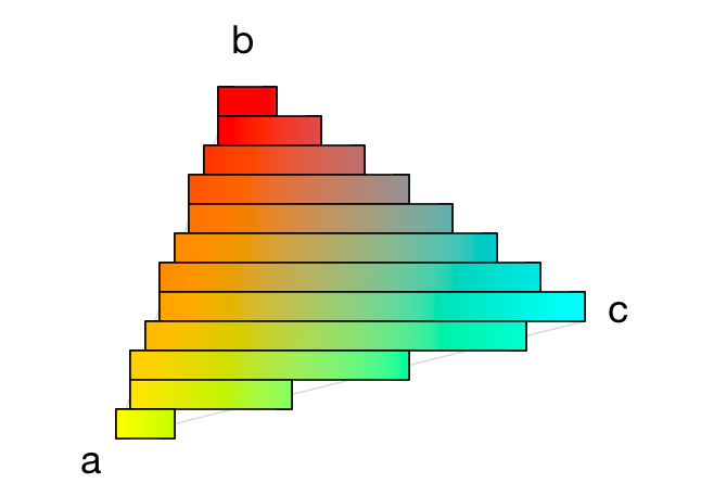
The same goes for the normal vector and the z-position: these are also interpolated going from the left Edge to the right Edge.

The code for drawSpans() looks like this:

func drawSpans() {
  if lastSpanLine != -1 {
    for y in firstSpanLine...lastSpanLine {
      if spans[y].edges.count == 2 {
        let edge1 = spans[y].leftEdge
        let edge2 = spans[y].rightEdge

        // How much to interpolate on each step.
        let step = 1 / Float(edge2.x - edge1.x)
        var pos: Float = 0

        for x in edge1.x ..< edge2.x {
          // Interpolate between the colors again.
          var r = edge1.r + (edge2.r - edge1.r) * pos
          var g = edge1.g + (edge2.g - edge1.g) * pos
          var b = edge1.b + (edge2.b - edge1.b) * pos
          let a = edge1.a + (edge2.a - edge1.a) * pos

          // Also interpolate the normal vector.
          let nx = edge1.nx + (edge2.nx - edge1.nx) * pos
          let ny = edge1.ny + (edge2.ny - edge1.ny) * pos
          let nz = edge1.nz + (edge2.nz - edge1.nz) * pos

          // TODO: depth buffer
          // TODO: draw the pixel

          pos += step
        }
      }
    }
  }
}

You can see how we step one pixel at a time from left to right and interpolate the color and the normal vector.

There’s more, which we’ll look at step-by-step.

First, there is the depth buffer. This is an array of Floats with the same dimension as the screen (800×600). The depth buffer makes sure that a triangle that is further away does not obscure a triangle that is closer to the camera.

This is done by storing the z-value of each triangle pixel into the depth buffer. We only draw the pixel if no “nearer” pixel has yet been drawn. That is, we only call setPixel() if the z-value is smaller than the z-value currently in the depth buffer at that position. (This is also a feature that Metal provides for you already.)

var shouldDrawPixel = true
if useDepthBuffer {
  let z = edge1.z + (edge2.z - edge1.z) * pos
  let offset = x + y * Int(context!.width)
  if depthBuffer[offset] > z {
    depthBuffer[offset] = z
  } else {
    shouldDrawPixel = false
  }
}

Finally, we can draw the pixel:

if shouldDrawPixel {
  let factor = min(max(0, -1*(nx*diffuseX + ny*diffuseY + nz*diffuseZ)), 1)

  r *= (ambientR*ambientIntensity + factor*diffuseR*diffuseIntensity)
  g *= (ambientG*ambientIntensity + factor*diffuseG*diffuseIntensity)
  b *= (ambientB*ambientIntensity + factor*diffuseB*diffuseIntensity)

  setPixel(x: x, y: y, r: r, g: g, b: b, a: a)
}

This is where the fragment shader does its job. It is called once for every pixel that we must draw, with interpolated values for the color, texture coordinates, normal vector, and so on. Here you can do all kinds of fun things.

In the demo app we calculate the color of the pixel based on a very simple lighting model, but you can also sample from a texture, or do lots of other wild things to the pixel color before it gets written into the framebuffer. You can make it as crazy as you can imagine it! 😎

Phew! That was a lot of effort just to get a rotating cube on the screen. To be fair, an API such as OpenGL or Metal does a lot more work than we’ve covered here — and much more efficiently — but this is conceptually what happens when you draw 3D objects using a GPU. I hope you found it enlightening!