YOLO: Core ML versus MPSNNGraph

A few weeks ago I wrote about YOLO, a neural network for object detection. I had implemented that version of YOLO (actually, Tiny YOLO) using Metal Performance Shaders and my Forge neural network library.

Since then Apple has announced two new technologies for doing machine learning on the device: Core ML and the MPS graph API. In this blog post we will implement Tiny YOLO with these new APIs.

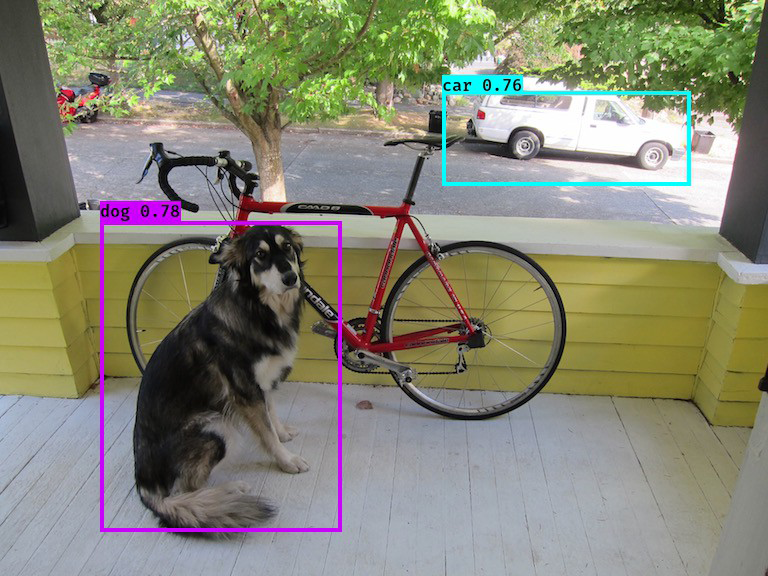
A quick recap: YOLO is a neural network made up of 9 convolutional layers and 6 max-pooling layers, but its last layer does not output a probability distribution like a classifier would. Instead the last layer produces a 13×13×125 tensor.

This output tensor describes a grid of 13×13 cells. Each cell predicts 5 bounding boxes (where each bounding box is described by 25 numbers). We then use non-maximum suppression to find the best bounding boxes.

As always, you can find the source code for this blog post on GitHub.

YOLO with Core ML

Let’s start with Core ML, since that is the framework most developers will want to use to put machine learning into their apps. To follow along, open the TinyYOLO-CoreML project in Xcode.

The first step is to create a .mlmodel file that describes the YOLO neural network.

The good news: the authors of YOLO have made a pre-trained network available, so we don’t have to do any training ourselves. 🎉

The bad news: it is in Darknet format. The Core ML conversion tools do not support Darknet, so we’ll first convert the Darknet files to Keras format. And then we can convert from Keras to Core ML.

Step 1: Darknet to Keras 1.2.2

In my previous YOLO post I used YAD2K to convert from Darknet to Keras 2.0. However, as I’m writing this the Core ML conversion tools only support Keras version 1.2.2. So first I had to hack the YAD2K scripts to use the older version of Keras (this hacked version of YAD2K is included in the repo).

You can find full instructions on how to do this conversion in the README file.

After the Darknet-to-Keras conversion succeeds, you’ll have the file tiny-yolo-voc.h5 (in the yad2k/model_data/ directory). This is the exact same model we used in the previous blog post, but compatible with Keras 1.2.2.

Step 2: Keras 1.2.2 to Core ML

Now that we have YOLO in a format that the Core ML conversion tools support, we can write a Python script to turn it into the .mlmodel file we need.

The Core ML conversion tools require Python 2.7, which already comes installed with macOS. Any other version of Python you may have installed will not work — you need to use the Python 2.7 from /usr/bin/python.

Since you’ll also need to install some packages, it’s best that you make a “virtualenv” or virtual environment. I’ll explain how to do that next.

First, make sure the Xcode 9 beta is installed and tell xcode-select to use this beta version for the command line tools. Run this command (and the ones that follow) from Terminal:

sudo xcode-select --switch /Applications/Xcode-beta.app/Contents/Developer

Also make sure you have pip installed. This is the Python package manager, and you’ll use it to install additional packages:

sudo easy_install pip

Next, install the virtualenv package:

pip install -U virtualenv

OK, that’s the preliminaries. Now we can create a virtual environment for Core ML. All the Python packages we’re going to install will be limited to just this virtual environment — they won’t clobber up your system folders. This is what allows us to run different versions of Python and Keras on the same system.

Here, we’ll put the virtual environment in the home folder (~ or /Users/yourname) but you can put it anywhere you like (just don’t move it afterwards or it will break).

Still in the Terminal, do:

cd ~
virtualenv -p /usr/bin/python2.7 coreml

The -p flag tells virtualenv to use the system version of Python 2.7. As I pointed out above, this is essential. If you use another Python version (even if it’s 2.7), the coremltools package will give errors.

source coreml/bin/activate

This activates the virtualenv you’ve just created. You’ll see that the terminal prompt now has (coreml) in front of it. That’s how you know which environment you’re in. (To return to the normal environment you can type the command deactivate.)

Now we can install the packages we need:

pip install tensorflow
pip install keras==1.2.2
pip install h5py
pip install coremltools

These packages will be installed in ~/coreml/lib/python2.7/site-packages/, so they go inside the folder from the virtualenv you’ve just set up.

Great, that concludes the setup. Now you can run the coreml.py conversion script (see the Convert folder in the repo). This reads the tiny-yolo-voc.h5 Keras model and writes TinyYOLO.mlmodel into the folder for the TinyYOLO-CoreML project.

This is what the coreml.py script looks like:

import coremltools

coreml_model = coremltools.converters.keras.convert(
    'yad2k/model_data/tiny-yolo-voc.h5',
    input_names='image',
    image_input_names='image',
    output_names='grid',
    image_scale=1/255.)

coreml_model.input_description['image'] = 'Input image'
coreml_model.output_description['grid'] = 'The 13x13 grid'

coreml_model.save('../TinyYOLO-CoreML/TinyYOLO-CoreML/TinyYOLO.mlmodel')

It’s a pretty simple script but it’s important to get the parameters correct in the call to coremltools.converters.keras.convert().

YOLO expects the pixels of the input image to be between 0 and 1, not 0 and 255, so we have to specify an image_scale of 1/255. There is no need for any other preprocessing on the input images.

You don’t need to run this conversion script yourself, as the repo already contains the TinyYOLO.mlmodel file, but in case you’re curious:

cd Convert
python coreml.py

The script prints out a bunch of information about the conversion process. At the end it prints out a summary of the model. It looks like this:

input {
  name: "image"
  shortDescription: "Input image"
  type {
    imageType {
      width: 416
      height: 416
      colorSpace: RGB
    }
  }
}
output {
  name: "grid"
  shortDescription: "The 13x13 grid"
  type {
    multiArrayType {
      shape: 125
      shape: 13
      shape: 13
      dataType: DOUBLE
    }
  }
}

This shows that YOLO expects an RGB image of size 416×416 pixels.

The output produced by this neural network is a “multi array” of shape 125×13×13. That makes sense. As you know, YOLO’s last layer outputs a grid of 13×13 cells and each cell contains 125 numbers that contain the predictions for 5 bounding boxes.

Excellent! After all this work we finally have a TinyYOLO.mlmodel file that we can stick into the app.

Step 3: Adding the model to the app

Adding a Core ML model into your app is a piece of cake: just drag-and-drop it into your Xcode project. Xcode then generates a source file that makes it really easy to talk to the model.

In our case Xcode has generated TinyYOLO.swift. This file does not appear in the Project Navigator, but you can click on TinyYOLO.mlmodel and from there view this source file.

We’re mostly going to be dealing with the TinyYOLO class:

@objc class TinyYOLO:NSObject {
    func prediction(image: CVPixelBuffer) throws -> TinyYOLOOutput {
        let input_ = TinyYOLOInput(image: image)
        return try self.prediction(input: input_)
    }
}

There’s more to this class but it’s mostly boilerplate. What we care about is the prediction(image) method. This method takes a CVPixelBuffer containing the image we want to analyze and returns a TinyYOLOOutput object.

class TinyYOLOOutput : MLFeatureProvider {
    let grid: MLMultiArray
}

The relevant part of this class is the MLMultiArray object. It contains our 13×13 grid of bounding box predictions. (The property is called grid because we specified this with the output_names='grid' parameter in the conversion script.)

Ideally, we would not use this TinyYOLO class directly, but through the Vision framework. Unfortunately, I was unable to get this to work (with beta 1 and 2).

We want Vision to give us a VNCoreMLFeatureValueObservation object, which in turn would contain the MLMultiArray with our 13×13 grid. But right now, Vision doesn’t actually return anything for this Core ML model. My guess is that support for things that aren’t classifiers doesn’t work very well yet in the current beta.

So for now we have no choice but to skip Vision and use Core ML directly. This means we need to put our input images into a CVPixelBuffer object somehow, and also resize this pixel buffer to 416×416 pixels — or Core ML won’t accept it.

Getting a CVPixelBuffer isn’t a big deal, since we’re using AVFoundation to capture live video and the AVCaptureVideoDataOutput delegate method can simply do the following:

public func captureOutput(_ output: AVCaptureOutput,
                          didOutput sampleBuffer: CMSampleBuffer, 
                          from connection: AVCaptureConnection) {

  let pixelBuffer = CMSampleBufferGetImageBuffer(sampleBuffer)
  // give the imageBuffer to Core ML ...
}

The CMSampleBufferGetImageBuffer() function takes the CMSampleBuffer object, which contains the pixel data from the camera, and turns it into a CVPixelBuffer.

However, the camera returns a 480×640 image, not 416×416, so we have to resize our camera output. No worries, Core Image to the rescue:

let ciImage = CIImage(cvPixelBuffer: pixelBuffer)
let sx = 416 / CGFloat(CVPixelBufferGetWidth(pixelBuffer))
let sy = 416 / CGFloat(CVPixelBufferGetHeight(pixelBuffer))
let scaleTransform = CGAffineTransform(scaleX: sx, y: sy)
let scaledImage = ciImage.transformed(by: scaleTransform)
ciContext.render(scaledImage, to: resizedPixelBuffer)

Since the camera image is taller than it is wide, this will squash the image a little. That’s not a big deal for this app, but you could use Core Image to first crop out the center square before resizing.

Now we have a CVPixelBuffer containing a 416×416 image that we can use to get predictions.

Step 4: Making predictions

Making a prediction is really easy with Core ML:

let model = TinyYOLO()

let image: CVPixelBuffer = ...

if let output = try? model.prediction(image: image) {
  // do something with output.grid
}

The output from model.prediction(image) is an MLMultiArray that describes the 13×13 grid.

Now how do we turn this into actual bounding boxes that we can show in the app?

The MLMultiArray object has dimensions 125×13×13. There are 125 channels for each cell in the 13×13 grid, because each cell predicts 5 bounding boxes and each bounding box is described by 25 numbers:

• 4 numbers for the coordinates of the rectangle
• 1 number for the confidence score (e.g. “I’m 75.3% sure this is a dog”)
• 20 numbers for the probabilities of the possible classes

The computeBoundingBoxes() function takes this MLMultiArray and converts it into a list of bounding boxes that we can draw on the screen. The math is actually 100% the same as in my previous blog post, so I’ll refer you there for the details.

I don’t want to show the entire function, only highlight the part that is different from the Metal version:

public func computeBoundingBoxes(features: MLMultiArray) -> [Prediction] {

  for cy in 0..<13 {
    for cx in 0..<13 {
      for b in 0..<5 {

        // Look at bounding box b for the grid cell (cy, cx):
        let channel = b*(numClasses + 5)
        let tx = features[[channel    , cy, cx] as [NSNumber]].floatValue
        let ty = features[[channel + 1, cy, cx] as [NSNumber]].floatValue
        let tw = features[[channel + 2, cy, cx] as [NSNumber]].floatValue
        let th = features[[channel + 3, cy, cx] as [NSNumber]].floatValue
        let tc = features[[channel + 4, cy, cx] as [NSNumber]].floatValue

        . . .
      }
    }
  }
}

To get the coordinates tx, ty, tw, th and the confidence score tc for a given bounding box, we have to subscript the MLMultiArray. Unfortunately, we can’t simply write:

let tx = features[channel, cy, cx]

Because MLMultiArray is really an Objective-C object, we need to wrap the indices in an array of NSNumber objects. The result is also an NSNumber, so we need to use .floatValue to turn it back into a Float.

I hope this is something that will get cleaned up in subsequent betas — all this NSNumber business is just plain ugly.

Step 5: Try it out!

Phew, that was a bit of work to get YOLO running on Core ML. But once you have done the model conversion, making predictions is pretty easy.

In the case of YOLO, just making the predictions isn’t enough. We still needed to do some extra processing on the output from the model, which involved working with the MLMultiArray class.

YOLO with MPSNNGraph

When you want to skip Core ML, or when Core ML doesn’t support your model type — or you just want to be hardcore — Metal is where you go.

In iOS 11 there are now two ways to use Metal Performance Shaders for machine learning:

1. create the MPSCNN kernels yourself and encode them into a command buffer (see my VGGNet post for an example)
2. describe your neural network using the new graph API and let the graph deal with everything

In this second part of the blog post, we’ll look at this new graph API. Does it really make things easier?

The code is in the TinyYOLO-NNGraph project, so open that to follow along.

Step 1: Converting the model

Yep, it starts with some converting here too. Again we’ll use the Keras 1.2.2 model created by YAD2K. (You could use Keras 2.0 for this but since I already made a 1.2.2 model for Core ML, we might as well use that one.)

In the previous YOLO post we created a conversion script that “folded” the batch normalization parameters into the weights of the convolution layers. That was needed because Metal does not have a batch normalization layer.

It still doesn’t… however, MPS can do this batch norm folding on your behalf now. So that makes the conversion script a lot simpler.

You can see the script in nngraph.py. Here’s a quick look:

import os
import numpy as np
import keras
from keras.models import Sequential, load_model

model_path = "yad2k/model_data/tiny-yolo-voc.h5"
dest_path = "../TinyYOLO-NNGraph/Parameters"

model = load_model(model_path)

def export_conv_and_batch_norm(conv_layer, bn_layer, name):
    bn_weights = bn_layer.get_weights()
    gamma = bn_weights[0]
    beta = bn_weights[1]
    mean = bn_weights[2]
    variance = bn_weights[3]

    conv_weights = conv_layer.get_weights()[0]
    conv_weights = conv_weights.transpose(3, 0, 1, 2).flatten()

    combined = np.concatenate([conv_weights, mean, variance, gamma, beta])
    combined.tofile(os.path.join(dest_path, name + ".bin"))

export_conv_and_batch_norm(model.layers[1], model.layers[2], "conv1")
export_conv_and_batch_norm(model.layers[5], model.layers[6], "conv2")
# and so on for the other layers ...

First this loads the tiny-yolo-voc.h5 model that we made with YAD2K.

Then it goes through all the convolution layers and puts the weights together with the batch normalization parameters into a single file, one file for each layer. There’s no requirement that you do this, but otherwise you end up with loads of tiny files. It also makes it easier to load this data in the app.

After running the conversion script we now have the files conv1.bin, conv2.bin, and so on. These files are placed into the TinyYOLO-NNGraph/Parameters folder and get copied by Xcode into the app bundle when you build the app.

Step 2: Adding the model to the app

One big change in the MPSCNN API is that when you create a new layer you no longer pass it an MPSCNNConvolutionDescriptor directly, nor do you give it the weights upon construction.

Instead, you need to give it an MPSCNNConvolutionDataSource object. This data source is responsible for loading the weights.

So let’s make our own data source. Since our layers are all very similar, we’re going to use the same DataSource class for all our layers — but each layer gets its own instance. The code looks like this:

class DataSource: NSObject, MPSCNNConvolutionDataSource {
  let name: String
  let kernelWidth: Int
  let kernelHeight: Int
  let inputFeatureChannels: Int
  let outputFeatureChannels: Int
  let useLeaky: Bool

  var data: Data?

  func load() -> Bool {
    if let url = Bundle.main.url(forResource: name, withExtension: "bin") {
      do {
        data = try Data(contentsOf: url)
        return true
      } catch {
        print("Error: could not load \(url): \(error)")
      }
    }
    return false
  }

  func purge() {
    data = nil
  }

  func weights() -> UnsafeMutableRawPointer {
    return UnsafeMutableRawPointer(mutating: (data! as NSData).bytes)
  }

  func biasTerms() -> UnsafeMutablePointer<Float>? {
    return nil
  }
}

The MPSCNNConvolutionDataSource protocol states that your data source should have load() and purge() functions. Here we simply load one of the binary files that we exported in the previous step (for example, conv1.bin) into a Data object.

To get the weights for this layer, the weights() function returns a pointer to the first element of this Data object. Our layers don’t have bias, so biasTerms() can return nil (this is typical when using batch norm, since the “beta” parameter already acts as a bias term).

The interesting part of the data source class is the function that returns the MPSCNNConvolutionDescriptor object:

func descriptor() -> MPSCNNConvolutionDescriptor {
  let desc = MPSCNNConvolutionDescriptor(
                   kernelWidth: kernelWidth,
                   kernelHeight: kernelHeight,
                   inputFeatureChannels: inputFeatureChannels,
                   outputFeatureChannels: outputFeatureChannels)

  desc.neuronType = .reLU
  desc.neuronParameterA = 0.1

  data?.withUnsafeBytes { (ptr: UnsafePointer<Float>) -> Void in
    let weightsSize = outputFeatureChannels * kernelHeight * 
                      kernelWidth * inputFeatureChannels
                      
    let mean = ptr.advanced(by: weightsSize)
    let variance = mean.advanced(by: outputFeatureChannels)
    let gamma = variance.advanced(by: outputFeatureChannels)
    let beta = gamma.advanced(by: outputFeatureChannels)
    
    desc.setBatchNormalizationParametersForInferenceWithMean(mean,
            variance: variance, gamma: gamma, beta: beta, epsilon: 1e-3)
  }

  return desc
}

With iOS 10 you would assign an MPSCNNNeuron object to the descriptor’s neuron property. This is now deprecated and you’re supposed to use the neuronType enum instead. Here we want to use a “leaky” ReLU, so we also set the value of neuronParameterA to 0.1.

Also new is the setBatchNormalizationParametersForInferenceWithMean() function. This makes it a lot easier to deal with batch normalization than before. Since we also store the mean, variance, gamma, and beta arrays in the Data object, we can just set the proper UnsafePointers and then call this method.

MPS will automatically deal with the batch normalization and we don’t have to worry about it anymore. Awesome!

Now that the data source is sorted out, we can start building our graph:

let inputImage = MPSNNImageNode(handle: nil)

let scale = MPSNNLanczosScaleNode(source: inputImage,
                 outputSize: MTLSize(width: 416, height: 416, depth: 3))

let conv1 = MPSCNNConvolutionNode(source: scale.resultImage,
                                  weights: DataSource("conv1", 3, 3, 3, 16))

let pool1 = MPSCNNPoolingMaxNode(source: conv1.resultImage, filterSize: 2)

let conv2 = MPSCNNConvolutionNode(source: pool1.resultImage,
                                  weights: DataSource("conv2", 3, 3, 16, 32))

let pool2 = MPSCNNPoolingMaxNode(source: conv2.resultImage, filterSize: 2)

// ... and so on ...

guard let graph = MPSNNGraph(device: device, 
                             resultImage: conv9.resultImage) else {
  fatalError("Error: could not initialize graph")
}

We start by declaring a node for the input image and a node that scales this input image to 416×416 pixels. Then follow the nodes for the network’s layers. Each layer is connected to the previous one using the source parameter. So the scale node is connected to inputImage, conv1 is connected to scale.resultImage, and so on. The graph itself is an MPSNNGraph object and is connected to the output of the very last layer in the network, conv9.

If you’ve used MPSCNN before, you’ll notice this is a lot less work to describe your neural network. However, some of the complexity has been moved into your data source object. If you have a complex network, then you may end up writing several different data source classes.

After I had first implemented YOLO using the graph API, I tried running the app and all the bounding boxes looked correct — except they were shifted down and to the right by 32 pixels. WTH?! After a bunch of debugging, it turned out that the padding on layer pool6 was wrong.

This pool6 layer is different from the other pooling layers in that it uses stride 1 instead of stride 2. And therefore it needs a different type of padding. To change how your layers are padded, you need to set the paddingPolicy property on the node. Like so:

pool6.paddingPolicy = MPSNNDefaultPadding(method: 
                   [.alignTopLeft, .addRemainderToBottomRight, .sizeSame])

By default the padding is set to .alignCentered instead of .alignTopLeft. This fixed the problem but the output of this pooling layer was not entirely correct yet, notably at the right side and bottom of the image.

At this point in the network, the image has been shrunk to 13×13 pixels, and since the filter is 2×2, there needs to be one pixel’s worth of padding at the right and bottom edges of the image.

It turns out that in my previous implementation I had set the edge mode for the padding kernel to “clamp” instead of “zero”. With zero, it adds zeros around the edge of the image (duh) but with clamp it duplicates the pixels. (Clamp tends to work better for max-pooling, especially if the values are likely to be negative.)

With the graph API there is no way to tell the max-pooling layer to use clamping instead of zeros. To do this you have to write your own class that implements the MPSNNPadding protocol.

Now, to be fair, YOLO would probably work just fine with zero padding instead of clamp padding, but as this whole exercise is about getting to know the graph API better, let’s make our own padding class. It looks something like this:

class Pool6Padding: NSObject, MPSNNPadding {
  func paddingMethod() -> MPSNNPaddingMethod {
    return [ .custom, .sizeSame ]
  }

  func destinationImageDescriptor(
                  forSourceImages sourceImages: [MPSImage],
                  sourceStates: [MPSState]?,
                  for kernel: MPSKernel,
                  suggestedDescriptor inDescriptor: MPSImageDescriptor) 
                  -> MPSImageDescriptor {
    if let kernel = kernel as? MPSCNNPooling {
      kernel.offset = MPSOffset(x: 1, y: 1, z: 0)
      kernel.edgeMode = .clamp
    }
    return inDescriptor
  }
}

There’s a bit more to it (having to do with NSCoding so that you can serialize the graph to a file) but these are the important parts. In paddingMethod() we return .custom. That will cause MPS to invoke the destinationImageDescriptor(...) function for this layer.

Inside this function we get access to the underlying MPSCNNPooling object, so that we can set its offset property to get the .alignTopLeft behavior, and also set its edgeMode to .clamp.

And now the graph computes the exact same result as the Forge version. 😀

Step 3: Making predictions

With Core ML the input image had to be a CVPixelBuffer but with Metal we want it to be an MTLTexture instead. Again, this is no biggie. In the camera code we can easily convert the pixels from the camera into a Metal texture:

if let imageBuffer = CMSampleBufferGetImageBuffer(sampleBuffer) {
  let width = CVPixelBufferGetWidth(imageBuffer)
  let height = CVPixelBufferGetHeight(imageBuffer)

  var texture: CVMetalTexture?
  CVMetalTextureCacheCreateTextureFromImage(kCFAllocatorDefault, textureCache,
         imageBuffer, nil, .bgra8Unorm, width, height, 0, &texture)

  if let texture = texture {
    let textureFromCamera = CVMetalTextureGetTexture(texture)
    // do a prediction using this texture...
  }
}

Once you have that texture, you only need to do the following to make a prediction using the graph:

let inputImage = MPSImage(texture: textureFromCamera, featureChannels: 3)

graph.executeAsync(withSourceImages: [inputImage]) { outputImage, error in
  if let image = outputImage {
    self.computeBoundingBoxes(image)
  }
}

The executeAsync() call takes care of all of the Metal stuff behind the scenes, and lets you know when it is done using the completion handler. Sweet!

In the completion handler we call computeBoundingBoxes(). This method is exactly the same as in my previous Metal implementation of YOLO, so I suggest you read that blog post for an explanation. (It’s also pretty much the same as what the Core ML version does, except that now the results are read from an MPSImage instead of an MLMultiArray.)

If your pipeline is more involved and requires custom kernels, then you can encode the graph into a command buffer yourself:

let commandBuffer = commandQueue.makeCommandBuffer()

// Run your own compute kernel for preprocessing
let myImageDesc = MPSImageDescriptor(...)
let myImage = MPSTemporaryImage(commandBuffer: commandBuffer, 
                                imageDescriptor: myImageDesc)
myComputeKernel.encode(commandBuffer: commandBuffer,
                       sourceTexture: textureFromCamera, 
                       destinationTexture: myImage.texture)

// Run the graph
let graphImg = graph.encode(to: commandBuffer, sourceImages: [myImage])

// Run your own postprocessing kernel
// ...

// This is called when the graph is finished
commandBuffer.addCompletedHandler { commandBuffer in
  // ...
}

commandBuffer.commit()

This way you can run your own compute kernels before or after the graph.

Step 4: Try it out!

Run the app and you should see… exactly the same as the Core ML version. No big surprise there as Core ML will use Metal under the hood.

Conclusion

I hope this blog post gave you some insight into the differences between working with Core ML and Metal’s graph API.

As for speed differences, it shouldn’t really matter. Both apps ought to run at comparable speeds and energy usage levels. However, in beta 1 the Core ML version is definitely slower. (I’m sure this will get better soon, since early betas are always on the slow side.)

The big difference between the two APIs is in ease-of-use. With Core ML it’s really easy to get your model up and running. With MPSNNGraph it takes more effort and you need to know more about the internals of the model. But both are definitely a lot easier to use than “old school” MPS.

The biggest downside of Core ML is that you get zero control over what happens when the model is running. But to be honest, even MPSNNGraph doesn’t really give you many options:

• It’s hard to understand what is going on inside the graph. You can do print(graph.debugDescription) to see what nodes are in the graph, what padding they are using, and so on. But there appears to be no way to inspect the graph for the image sizes that it automatically infers.

• You can’t extend the graph API to add custom kernels. It is possible to run your own kernels before or after the graph, or to split the graph into two parts and do your own work in the middle. However, if you want to use a custom kernel throughout the network, the graph API cannot help you.

This last point is a major downside. With Core ML you depend on the mlmodel format specification — if some part of your model isn’t supported by Core ML, you can’t use this API. But the same thing is true for MPSNNGraph: if your model needs to do something that isn’t included in MPS, you can’t use the graph API.

I think Core ML is a great solution for when you have a simple model or want to use a proven deep learning model that has been around for a while.

But if you want to be on the forefront of deep learning, you’ll have to go low-level and use Metal. And if that means you need to use custom compute kernels, then MPSNNGraph is not an option for you. You can still use Metal but you’ll have to create your network the hard way.